Blog

  • Master AI Agent Automation with RAG on Gradient Platform

    Master AI Agent Automation with RAG on Gradient Platform

    Introduction

    Building an AI agent with RAG on the Gradient Platform transforms how teams handle compliance automation. This innovative approach uses Retrieval-Augmented Generation (RAG) to automate complex security and compliance questionnaires, cutting manual effort by up to 90%. By integrating AI-driven document retrieval and contextual response generation, the system ensures faster, more consistent, and accurate results for SaaS companies. In this guide, you’ll learn how to create, deploy, and scale an AI-powered workflow that streamlines enterprise compliance with precision and speed.

    What is AI-Powered Security Questionnaire Automation?

    This solution helps companies automatically answer long and repetitive security and compliance questionnaires using artificial intelligence. It reads a company’s existing security and privacy documents, understands the questions, and generates accurate and consistent answers in much less time than manual work. The goal is to save hours of effort, speed up business processes, and ensure reliable, well-documented responses without needing technical or compliance experts to do everything by hand.

    Who Needs This Solution

    Picture this, you’re part of a SaaS company growing faster than you can grab another cup of coffee. Every new client means another batch of those long and repetitive security and compliance questionnaires. They’re important, sure, but they can also make your whole team groan together. That’s where this AI-powered solution comes in, like a superhero that saves the day for productivity.

    It’s built for SaaS companies that are scaling fast and constantly being checked by security auditors. You know how it goes, every new deal or partnership means another checklist, and your compliance team feels buried under endless documents. With this solution, they can finally breathe because the AI takes care of the repetitive stuff quickly, accurately, and without all the stress.

    If you’re on a compliance or security team, you’ll love how it automates the tasks that eat up most of your time. Imagine focusing on the big, important projects instead of searching through documents for the hundredth time. Even your sales and business development teammates will be happy about it because it helps them close deals faster by cutting down those annoying delays caused by pending compliance questions.

    And if you’re part of a startup? This is a total lifesaver. When every minute and dollar matters, this tool lets you handle compliance like a big company without needing a big team or huge budget. It’s like adding a full compliance department to your crew without actually hiring one.

    Benefits of AI-Powered Questionnaire Automation

    Let’s chat about what makes this solution so good.

    • Time Efficiency: Imagine shrinking your security questionnaire work from several days to just a few hours. That’s not magic, that’s automation doing the heavy lifting.
    • Consistency: This solution ensures that every answer stays consistent and follows your company’s standards, meaning fewer mistakes and no last-minute rewrites.
    • Resource Optimization: Your developers shouldn’t waste time filling out compliance forms—they should be coding! The AI handles the boring documentation.
    • Scalability: As your company grows and questionnaires pile up, this system scales smoothly without needing more hires.
    • Accuracy: The AI uses real data from verified company documents, ensuring every answer is evidence-backed.

    Here’s where it gets interesting: you’ll actually learn how to build your own AI-powered app using Retrieval-Augmented Generation (RAG). It helps your AI “read” and “understand” your company’s documents to write smart, accurate answers—cutting response time by up to 80%.

    Prerequisites

    Before we jump into the hands-on part, make sure you have a Caasify account. You should also know a bit about RAG, APIs, and how modern web apps work. If you’ve used Streamlit, Docker, or Python 3.10, you’re good to go. You’ll also need access to the Caasify Gradient Platform where your AI agent will operate.

    Step-by-Step Guide to Building an AI-Powered Security Questionnaire App

    You’ll start by creating an AI agent in the Caasify Gradient Platform, then set up a secure private endpoint. Next, build a Streamlit + Python app to process Excel files, and finally deploy everything to a cloud platform.

    Why is an AI Agent Needed for Security Questionnaire Automation

    An AI agent is your perfect sidekick—it never gets tired and thrives on complexity. It reads questionnaires, finds answers from your policies, and writes accurate responses. This means fewer errors and faster results.

    These questionnaires cover topics like Data Protection, Access Controls, Network Security, and compliance frameworks like:

    • GDPR: EU privacy law regulating data handling.
    • HIPAA: U.S. healthcare information privacy law.
    • SOC 2: Ensures secure and responsible data management.
    • ISO 27001: Global information security standard.
    • NIST: Cybersecurity framework for risk management.
    • DPDP: India’s digital data protection law.

    With automation via Caasify Gradient and RAG, your AI agent can answer these in minutes instead of days—accurately and consistently.

    High Level Design of Gradient Platform

    The Gradient Platform manages data pipelines, embedding models, APIs, and user interfaces. It’s the unseen powerhouse enabling your AI agent to process documents efficiently.

    High Level Design of Application

    The Streamlit front-end provides an interface for uploading questionnaires, while backend APIs communicate with the AI agent. It’s a scalable and modular architecture that’s easy to maintain.

    Hands-On Tutorial

    Prefer watching instead? A demo video walks through every step, showing the AI agent answering questions in real time.

    Step 1 – Creating the GenAI Agent

    Collect compliance documents (like ISO, SOC 2, privacy policies) and format them as Markdown or plain text. Upload or link them in your Caasify Gradient Platform under the Knowledge Base section.

    Use OpenSearch as your vector database, choose a lightweight multilingual embedding model, and run indexing. Then create your GenAI Agent using a foundation model like LLaMA 3 8B. Connect your knowledge base, set the system prompt to return JSON responses, and deploy it.

    Step 2 – Configuring the Private Endpoint

    Generate a private API key under “Endpoint Access Keys” and save it in your environment variables along with your endpoint URL for secure communication.

    Step 3 – Building the Streamlit + Python App

    Create a GitHub repository for your project and structure it like this:

    project/
    ├── app.py        # Main Streamlit app
    ├── chatbot.py   # Backend logic for API calls
    ├── requirements.txt # Python dependencies
    ├── Dockerfile         # For deployment

    The chatbot.py handles AI communication:

    import os
    import requests
    from dotenv import load_dotenvload_dotenv()
    AGENT_ENDPOINT = os.getenv(“AGENT_ENDPOINT”) + “/api/v1/chat/completions”
    AGENT_ACCESS_KEY = os.getenv(“AGENT_ACCESS_KEY”)def ask_question(question):
        prompt = base_prompt + “nQuestion: ” + question
        payload = {
            “messages”: [{ “role”: “user”, “content”: prompt }]
        }
        headers = {
            “Content-Type”: “application/json”,
            “Authorization”: f”Bearer {AGENT_ACCESS_KEY}”
        }
        response = requests.post(AGENT_ENDPOINT, json=payload, headers=headers)
        return response.json()

    The app.py handles file upload and processing:

    import pandas as pd
    import jsondef process_security_questions(uploaded_file):
        try:
            df = pd.read_excel(uploaded_file)
            question_col_index = None
            for i, col in enumerate(df.columns):
                if ‘question’ in str(col).lower():
                    question_col_index = i
                    break
            if question_col_index is None:
                st.error(“Could not find a column containing ‘question’”)
                return None
            answers = []
            progress_bar = st.progress(0)
            num_rows = len(df)
            for i in range(num_rows):
                question = str(df.iloc[i, question_col_index])
                response = ask_question(question)
                try:
                    content = response[“choices”][0][“message”][“content”]
                    answer_data = json.loads(content)
                except Exception as e:
                    answer_data = { “answer”: “Not Sure”, “reasoning”: “Failed” }
                answers.append(answer_data)
            df[“Answer”] = [a.get(“answer”, “”) for a in answers]
            df[“Reasoning”] = [a.get(“reasoning”, “”) for a in answers]
            return df
        except Exception as e:
            st.error(f”Error: {str(e)}”)
            return None

    Your Dockerfile for deployment:

    FROM python:3.11-slim-buster
    WORKDIR /app
    COPY . ./app
    COPY requirements.txt ./
    RUN pip3 install -U pip && pip3 install -r requirements.txt
    CMD [“streamlit”, “run”, “app/app.py”]

    Step 4 – Deploying the App on the Caasify App Platform

    Connect your GitHub repo to Caasify, select your branch and Dockerfile, set AGENT_ENDPOINT and AGENT_ACCESS_KEY environment variables, then deploy. Choose an instance size and region, and your AI agent will be live in minutes.

    Testing the Application

    Once live, upload an Excel file with security questions and click Process Questions. The AI will generate answers with explanations. Review them, download your CSV, and enjoy the saved time.

    FAQs

    1. What types of questionnaires work best? Structured Excel-based ones like SOC 2, ISO 27001, and GDPR.
    2. How accurate are the answers? Around 85% with a well-prepared knowledge base.
    3. Can I customize the AI tone? Yes, edit the prompts to match your company’s tone and style.
    4. Can I attach documents? The AI can suggest attachments; you’ll need to handle them manually.
    5. Is my data safe? Yes, it stays within your Caasify environment, under your full control.
    6. How much time does it save? 70–90% time savings for most teams.
    7. Can it integrate with other systems? Absolutely—connects with CRMs, ticketing tools, and document platforms via APIs.
    8. What setup is needed? A solid cloud platform like Caasify Gradient for best performance. Learn more from IBM Research RAG Overview.

    Conclusion

    Mastering AI agent automation with RAG on the Gradient Platform is a powerful step toward smarter, faster compliance management. By combining Retrieval-Augmented Generation (RAG) with an AI-driven workflow, businesses can automate repetitive security and compliance questionnaires, improving accuracy and cutting turnaround times dramatically. This approach not only boosts productivity but also ensures consistent, reliable responses that align with enterprise-level standards.As AI agents continue to evolve, their integration with platforms like the Gradient Platform will reshape how organizations handle compliance, documentation, and workflow automation. Future advancements in LLMs and RAG models will bring even greater efficiency, deeper contextual understanding, and more scalable enterprise solutions.In short, AI-powered automation is redefining compliance operations—streamlining processes, enhancing precision, and helping teams stay ahead in a rapidly transforming digital landscape.

    Cloud-Based RAG System Setup: Essential Requirements for Deployment and Scalability (2025)

  • Master Data Augmentation for Object Detection with Rotation and Shearing

    Master Data Augmentation for Object Detection with Rotation and Shearing

    Introduction

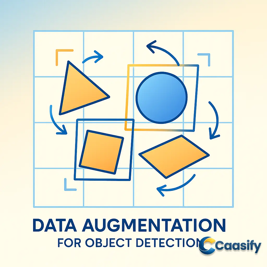
    Mastering data augmentation for object detection with rotation and shearing is key to building smarter, more resilient AI models. In computer vision, data augmentation enhances training datasets by introducing geometric transformations that simulate real-world diversity. Rotation adjusts image orientation, while shearing skews perspective—both requiring precise updates to bounding boxes for accuracy. This guide explores how these techniques strengthen model performance, reduce overfitting, and improve object recognition across varied environments.

    What is Data augmentation using rotation and shearing?

    This solution involves expanding and improving image datasets by slightly changing existing pictures. It works by rotating images or slanting them at angles to make a computer model better at recognizing objects from different perspectives. Instead of collecting thousands of new photos, this method teaches the system to understand variations in shape, angle, and position, making object detection more accurate and reliable in real-world situations.

    Prerequisites

    Before we get into the world of bounding box augmentation with rotation and shearing, let’s make sure you’ve got the basics covered. Think of this as checking your gear before a hike on a new trail. These concepts will make your work smoother and a lot more fun. You know, data augmentation might seem tricky at first, but once you understand the basics, everything starts to fall into place. So, let’s go over what you’ll need to know before we start working with those bounding boxes.

    First, you’ll need a simple understanding of image augmentation. If you’ve worked with computer vision before, you probably already know that transformations like rotation, flipping, scaling, and translation are the core parts of data augmentation. For example, rotation spins your image around a point, which helps your model recognize objects from different angles. Flipping gives your image a mirror effect, which is great for learning symmetry. Scaling zooms in or out to change the size, while translation moves the image around the frame. These steps might sound straightforward, but together, they make your dataset much richer. This helps prevent overfitting and makes your model perform better on new, unseen data. Once you understand what each transformation really does, you can use them wisely, rather than just tossing them in and hoping for the best.

    Next, let’s talk about bounding boxes. These are the rectangular outlines that show where objects are inside your image. Picture tagging a car in a photo—your bounding box is that rectangle around it, defined by four coordinates, (x_min, y_min, x_max, y_max). Here, x_min and y_min mark the top-left corner, while x_max and y_max define the bottom-right one. Pretty simple, right? But here’s the catch: when you apply data augmentation, it’s not just the image that changes—the bounding boxes have to change too. If your image rotates or shears but your boxes stay still, the labels won’t match anymore, and your object detection model will start learning the wrong thing. So, knowing how to move these coordinates correctly after every transformation is key to keeping your annotations right where they should be.

    Now, to handle these transformations the right way, you’ll need a basic idea of coordinate geometry. Don’t worry, we’re not diving into heavy math here. You just need to know how points, lines, and shapes move when they’re rotated, shifted, or scaled on a grid. For example, when you rotate an image, every pixel and bounding box corner moves based on trigonometric functions like sine and cosine. It’s kind of like choreographing a dance where every point knows exactly how to move to stay in rhythm. Understanding this helps you calculate new bounding box positions after transformations so that everything stays perfectly aligned.

    And finally, let’s talk about the tools that make this all possible—Python and NumPy. Python is your main language for computer vision because it has libraries that make image processing easy to handle. NumPy, on the other hand, is your math buddy behind the scenes. It lets you handle arrays and matrices quickly, which are super important when transforming images or coordinates. You’ll use Python and NumPy to build transformation matrices, apply them to images, and update bounding box coordinates. Knowing how to reshape arrays, multiply matrices, and do quick element-wise math will save you a ton of time and frustration.

    So, before you dive deep into rotation, shearing, and other data augmentation tricks, make sure you’re comfortable with these four essentials—image augmentation basics, bounding box handling, coordinate geometry, and Python with NumPy. Each one plays an important part in building strong, realistic, and correctly labeled datasets. Once you’ve got them nailed down, you’ll be ready to build object detection models that are not just smart but flexible—the kind that can handle real-world images from any angle or shape.

    TensorFlow Data Augmentation Guide

    GitHub Repo

    You know how every good project needs a home base, a spot where all your hard work lives, well-organized and easy to find? That’s exactly what this GitHub repository is meant to be. It’s not just a bunch of code files tossed together, it’s the main hub of this whole data augmentation journey. Inside, you’ll find everything we’ve covered, like rotation, shearing, and those complex bounding box transformations, all neatly packed into one clean, easy-to-navigate library.

    Think of it like a workshop where every tool sits right where it should. The repository holds all the scripts, each one clearly labeled and explained so you can dive in without getting lost. You’ll see step-by-step examples that show you how to use transformations like image rotation and shearing to expand your dataset for object detection tasks. Want to test out scaling or play around with different image angles? It’s all there, clearly arranged for you to explore.

    Here’s a clearer way to say it: the code isn’t just something to copy and paste—it’s there for you to experiment with. Every script is set up so you can adjust parameters, test new ideas, or even build creative combinations of augmentations. Whether you’re experimenting with various shearing intensities or tweaking how your bounding boxes respond to rotation, this repo gives you the perfect place to learn by doing.

    And there’s more. The library also includes ready-to-use helper functions designed to make your work smoother. Think of these as your quiet support team, taking care of the heavy-lifting math like generating transformation matrices, fixing bounding box coordinates, and keeping your image geometry accurate after every transformation. That way, you can focus on the creative part—building better and smarter data workflows—without getting stuck in the details of coordinate math.

    By exploring these scripts, you’ll start to see how each data augmentation technique, whether it’s a small rotation, a bold shear, or a clever mix of both, helps your model view the world from different angles. This understanding is key to improving how well your model performs and adapts in real-world settings. It’s like teaching your model to recognize something whether it’s upside down, sideways, or just a little skewed.

    If your aim is to create an object detection model that holds up under any condition, this GitHub repo is your complete toolkit. You can try out different data augmentation parameters, check how they affect your dataset, and fine-tune everything until your model gets that satisfying “aha!” moment of accuracy.

    So now that all the tools are ready to go—the rotation scripts, the shearing logic, the bounding box helpers—it’s time to roll up your sleeves and dig in. Let’s see how these transformations can take ordinary data and turn it into powerful training fuel for your next big object detection breakthrough, Data Augmentation Overview (Papers with Code).

    Rotation

    Ah, rotation, the bold move of data augmentation. At first, it seems simple enough, right? Just spin the image a bit and keep going. But, as you’ll quickly find out, rotation hides a lot of geometry behind the scenes, especially when you’re trying to keep those bounding boxes accurate. It’s one of those steps that looks easy until you realize it’s been quietly reshaping your data in ways you didn’t plan for.

    Let’s start with something that might sound fancy but actually makes perfect sense once you picture it: the Affine Transformation. Think of it as the invisible rulebook that tells an image how to move without messing up its shape. You can stretch it (scaling), slide it (translation), or spin it (rotation), but no matter what, the parallel lines stay parallel. That’s why affine transformations matter so much in data augmentation. They copy how the world looks when you move around it, giving your object detection model new viewpoints to learn from.

    Now, here’s where it gets interesting. How do we actually make this happen in code? This is where our main tool, the transformation matrix, steps in. It’s like a mathematical remote control that tells every point in your image exactly where to go. Imagine each pixel as a tiny dot on a map. The matrix tells each one how to move to its new position. You don’t need to turn into a math expert for this, but it helps to know that when you multiply your coordinates [x, y] with this matrix, you get a brand-new set of coordinates showing where that point lands after the move.

    This 2×3 matrix works together with a little 3×1 vector [x, y, 1]. That extra “1” helps keep translations smooth. Together, they handle rotation, scaling, and translation. These are the moves that make data augmentation work so well. When you rotate, you can even pick the exact spot to spin around, usually the center of the image.

    Here’s a clearer way to say it: you don’t need to do the math yourself. Libraries like OpenCV do all the work for you. Its cv2.warpAffine() function is like your all-in-one transformation helper. You just pass it your matrix, and it returns a perfectly rotated image.

    Now that the theory is out of the way, let’s get our hands dirty with some code. We’ll start with a simple __init__ function:

    def __init__(self, angle = 10):
        self.angle = angle
        if type(self.angle) == tuple:
            assert len(self.angle) == 2, “Invalid range”
        else:
            self.angle = (-self.angle, self.angle)

    This bit of code sets how much rotation you want, either a specific angle or a random range for a bit of variety.

    Next, we actually rotate the image. The goal here is to spin it around its center using OpenCV’s cv2.getRotationMatrix2D() function. Here’s how it looks:

    (h, w) = image.shape[:2]
    (cX, cY) = (w // 2, h // 2)
    M = cv2.getRotationMatrix2D((cX, cY), angle, 1.0)

    Here, cX and cY mark the center of the image, and M is our transformation matrix. Once that’s ready, we use cv2.warpAffine() to make it happen:

    image = cv2.warpAffine(image, M, (w, h))

    This rotates the image nicely, but there’s one catch. When you spin the image, some parts might stretch beyond the original frame. OpenCV, being practical, just chops those parts off, which means you lose some edges. Not ideal, right?

    So, how do we fix this? A bit of trigonometry saves the day. We calculate the new width and height that the rotated image needs to keep everything visible:

    cos = np.abs(M[0, 0])
    sin = np.abs(M[0, 1])
    nW = int((h * sin) + (w * cos))
    nH = int((h * cos) + (w * sin))

    These formulas make enough room for every corner of the image, no matter how it’s rotated. But now the image’s center has shifted, so we fix that by adjusting the matrix:

    M[0, 2] += (nW / 2) – cX
    M[1, 2] += (nH / 2) – cY

    This tweak keeps the rotated image centered and complete, so you don’t lose anything.

    Now, we’ll wrap it all into a neat function called rotate_im:

    def rotate_im(image, angle):
        “””Rotate the image.
        Rotate the image such that the rotated image is enclosed inside the tightest rectangle.
        The area not occupied by the pixels of the original image is colored black.
        “””
        (h, w) = image.shape[:2]
        (cX, cY) = (w // 2, h // 2)
        M = cv2.getRotationMatrix2D((cX, cY), angle, 1.0)
        cos = np.abs(M[0, 0])
        sin = np.abs(M[0, 1])
        nW = int((h * sin) + (w * cos))
        nH = int((h * cos) + (w * sin))
        M[0, 2] += (nW / 2) – cX
        M[1, 2] += (nH / 2) – cY
        image = cv2.warpAffine(image, M, (nW, nH))
        return image

    This function makes sure your rotated image stays fully visible and well-centered.

    Now, rotating an image is one thing, but rotating the bounding boxes is where it gets tricky. Each bounding box defines where your object sits, and when the image turns, those boxes have to turn too. If they don’t, your data augmentation might send your object detection model off track.

    We start by grabbing the coordinates of all four corners of each bounding box:

    def get_corners(bboxes):
        “””Get corners of bounding boxes”””
        width = (bboxes[:,2] – bboxes[:,0]).reshape(-1,1)
        height = (bboxes[:,3] – bboxes[:,1]).reshape(-1,1)
        x1 = bboxes[:,0].reshape(-1,1)
        y1 = bboxes[:,1].reshape(-1,1)
        x2 = x1 + width
        y2 = y1
        x3 = x1
        y3 = y1 + height
        x4 = bboxes[:,2].reshape(-1,1)
        y4 = bboxes[:,3].reshape(-1,1)
        corners = np.hstack((x1,y1,x2,y2,x3,y3,x4,y4))
        return corners

    Once we have those corners, we rotate them using the same transformation matrix:

    def rotate_box(corners, angle, cx, cy, h, w):
        “””Rotate the bounding box.”””
        corners = corners.reshape(-1,2)
        corners = np.hstack((corners, np.ones((corners.shape[0],1), dtype=type(corners[0][0]))))
        M = cv2.getRotationMatrix2D((cx, cy), angle, 1.0)
        cos = np.abs(M[0, 0])
        sin = np.abs(M[0, 1])
        nW = int((h * sin) + (w * cos))
        nH = int((h * cos) + (w * sin))
        M[0, 2] += (nW / 2) – cx
        M[1, 2] += (nH / 2) – cy
        calculated = np.dot(M, corners.T).T
        calculated = calculated.reshape(-1,8)
        return calculated

    After rotation, the boxes tilt slightly, so we calculate a new enclosing rectangle that wraps around them perfectly:

    def get_enclosing_box(corners):
        “””Get an enclosing box for rotated corners of a bounding box”””
        x_ = corners[:,[0,2,4,6]]
        y_ = corners[:,[1,3,5,7]]
        xmin = np.min(x_,1).reshape(-1,1)
        ymin = np.min(y_,1).reshape(-1,1)
        xmax = np.max(x_,1).reshape(-1,1)
        ymax = np.max(y_,1).reshape(-1,1)
        final = np.hstack((xmin, ymin, xmax, ymax, corners[:,8:]))
        return final

    Finally, we put it all together in the __call__ function:

    def __call__(self, img, bboxes):
        angle = random.uniform(*self.angle)
        w,h = img.shape[1], img.shape[0]
        cx, cy = w//2, h//2
        img = rotate_im(img, angle)
        corners = get_corners(bboxes)
        corners = np.hstack((corners, bboxes[:,4:]))
        corners[:,:8] = rotate_box(corners[:,:8], angle, cx, cy, h, w)
        new_bbox = get_enclosing_box(corners)
        scale_factor_x = img.shape[1] / w
        scale_factor_y = img.shape[0] / h
        img = cv2.resize(img, (w,h))
        new_bbox[:,:4] /= [scale_factor_x, scale_factor_y, scale_factor_x, scale_factor_y]
        bboxes = new_bbox
        bboxes = clip_box(bboxes, [0,0,w, h], 0.25)
        return img, bboxes

    And just like that, rotation—one of the toughest parts of data augmentation—turns into a powerful and reliable tool. With rotation and bounding boxes working in harmony, your object detection model can finally view the world from every possible angle. For more details, visit the OpenCV Image Transformations Guide.

    Rotating the Image

    Alright, let’s talk about one of the coolest and most useful tricks in data augmentation, rotation. You’ve probably rotated an image before, maybe to straighten a tilted picture or make it look a bit more interesting. But here’s the thing, when it comes to object detection, rotation isn’t just about style. It’s all about math, geometry, and precision working together.

    So, the first thing you need to do is spin your image around its center, kind of like giving it a neat twirl, by a specific angle θ (theta). To make that happen, we use something called a transformation matrix. Think of it like a set of rules that tells each pixel where to go to pull off that perfect spin.

    Luckily, we don’t have to figure out the math by hand because OpenCV already has a built-in helper called getRotationMatrix2D. It does the hard part for us. Here’s what it looks like:

    (h, w) = image.shape[:2]
    (cX, cY) = (w // 2, h // 2)
    M = cv2.getRotationMatrix2D((cX, cY), angle, 1.0)

    Here, h and w are just the image’s height and width, while (cX, cY) marks the center point where the rotation happens. It’s like finding the middle of a spinning record before hitting play.

    The function cv2.getRotationMatrix2D() builds a 2×3 affine transformation matrix, M, which takes care of both rotation and translation in one go. The last part, 1.0, is the scaling factor, which keeps your image size the same so it doesn’t accidentally zoom in or out during the rotation.

    Once the transformation matrix is ready, we use another OpenCV tool called warpAffine to actually apply it:

    image = cv2.warpAffine(image, M, (w, h))

    That (w, h) part simply tells OpenCV what the size of the output image should be. But here’s a little catch. When you rotate an image, some parts might extend beyond the original frame. Think of it like spinning a rectangular piece of paper—the corners will poke out past the edges. OpenCV, being tidy, just trims those parts off. Yep, it crops them, and that means you lose some data along the edges.

    This common issue is known as the OpenCV rotation side-effect. It’s like losing a bit of the corners in your photo because you didn’t give it enough space to rotate freely.

    The fix? You give your image a bigger “canvas,” basically a new bounding box that can hold the entire rotated image without chopping off any parts.

    To figure out the new size, we use a bit of trigonometry. When you rotate a rectangular image by an angle θ, the new width and height (we’ll call them nW and nH) can be calculated like this:

    cos = np.abs(M[0, 0])
    sin = np.abs(M[0, 1])
    nW = int((h * sin) + (w * cos))
    nH = int((h * cos) + (w * sin))

    Here’s what’s happening. The cosine and sine of the angle tell us how much each corner moves horizontally and vertically. We take the absolute values because negative lengths don’t make sense here. These formulas make sure the new bounding box is big enough to hold the rotated image completely.

    But wait, there’s one more small fix to make. Since the image now has a new size, its center changes a bit too. To keep the rotation centered, we need to tweak the translation values in our transformation matrix:

    M[0, 2] += (nW / 2) – cX
    M[1, 2] += (nH / 2) – cY

    This adjustment keeps the image centered after rotation so nothing slides off to one side. It’s like repositioning your coffee cup after spinning it—it’s still centered, just inside a slightly larger circle.

    Now that we’ve worked out all the math, let’s wrap it up neatly in a reusable function called rotate_im. Here’s the complete code:

    def rotate_im(image, angle):
        “””
        Rotate the image.
        Rotate the image such that the rotated image is enclosed inside the tightest
        rectangle. The area not occupied by the pixels of the original image is colored
        black.
        “””
        # grab the dimensions of the image and then determine the center
        (h, w) = image.shape[:2]
        (cX, cY) = (w // 2, h // 2)    # grab the rotation matrix (applying the negative of the angle
        # to rotate clockwise), then grab the sine and cosine
        M = cv2.getRotationMatrix2D((cX, cY), angle, 1.0)
        cos = np.abs(M[0, 0])
        sin = np.abs(M[0, 1])    # compute the new bounding dimensions of the image
        nW = int((h * sin) + (w * cos))
        nH = int((h * cos) + (w * sin))    # adjust the rotation matrix to take into account translation
        M[0, 2] += (nW / 2) – cX
        M[1, 2] += (nH / 2) – cY    # perform the actual rotation and return the image
        image = cv2.warpAffine(image, M, (nW, nH))
        # image = cv2.resize(image, (w, h))
        return image

    Here’s a clearer way to say what this function does. It finds the image’s center so it knows where to rotate from. Then it creates a rotation matrix using the chosen angle and scaling factor. Next, it calculates the new image size to make sure no part gets left out. After that, it adjusts the matrix translation so the image stays centered, and finally, cv2.warpAffine() applies the transformation to produce the rotated image.

    The best part? The rotated image fits perfectly inside its new frame—no cropping, no data loss, and any extra space around the edges (caused by rotation) gets filled with black pixels, keeping the final image neat and clean.

    And just like that, we’ve turned a simple rotation into a precise, geometry-backed transformation. This step is crucial for object detection because it helps models learn how to recognize objects from different angles. It’s a small yet powerful move in data augmentation, giving your models the ability to handle images that are turned, tilted, or even flipped in real-world situations.

    If you want to explore more about how to rotate images and translations in OpenCV, check out Image Rotation and Translation using OpenCV.

    Rotating the Bounding Box

    Now, this is where things get a bit more interesting in the world of data augmentation, OpenCV Geometric Transformations rotating the bounding boxes. It’s not just about spinning an image and calling it done. This step takes some accuracy, a bit of math, and a steady hand. Think of it like tossing a pizza box in the air, you’ve got to make sure the toppings don’t slide off halfway through the spin.

    When you rotate an image, the bounding boxes around the objects, those neat rectangles that guide object detection, also tilt with it. Suddenly, your nice upright rectangle turns into a diagonal shape. To fix that, you have to redraw a new, upright rectangle that still wraps perfectly around the tilted one. It’s kind of like adjusting a photo frame so it fits a picture that’s been turned at an angle without cutting off any part of it.

    So, how do we make that work? First, we grab all the coordinates of the original bounding box corners. Sure, you could technically use just two corners (the top-left and bottom-right), but doing it that way would turn into a complicated trigonometry session. Instead, it’s easier and much more accurate to use all four corners. That gives you the complete geometry of the box, which makes everything smoother later on.

    Here’s the little helper function that does the trick inside bbox_utils.py:

    def get_corners(bboxes):     “””Get corners of bounding boxes”””     width = (bboxes[:,2] – bboxes[:,0]).reshape(-1,1)     height = (bboxes[:,3] – bboxes[:,1]).reshape(-1,1)     x1 = bboxes[:,0].reshape(-1,1)     y1 = bboxes[:,1].reshape(-1,1)     x2 = x1 + width     y2 = y1     x3 = x1     y3 = y1 + height     x4 = bboxes[:,2].reshape(-1,1)     y4 = bboxes[:,3].reshape(-1,1)     corners = np.hstack((x1,y1,x2,y2,x3,y3,x4,y4))     return corners

    After this function runs, every bounding box now has eight coordinate values, one pair for each corner: (x1, y1), (x2, y2), (x3, y3), and (x4, y4). Now that we’ve got those points, it’s time to rotate them.

    To keep things consistent, we rotate these corners using the same transformation matrix we used for the image itself. That’s how we make sure the boxes stay perfectly aligned with the rotated image, without slipping out of place. Here’s the function that handles that: rotate_box

    def rotate_box(corners, angle, cx, cy, h, w):     “””Rotate the bounding box.”””     corners = corners.reshape(-1,2)     corners = np.hstack((corners, np.ones((corners.shape[0],1), dtype = type(corners[0][0]))))     M = cv2.getRotationMatrix2D((cx, cy), angle, 1.0)     cos = np.abs(M[0, 0])     sin = np.abs(M[0, 1])     nW = int((h * sin) + (w * cos))     nH = int((h * cos) + (w * sin))     # adjust the rotation matrix to take into account translation     M[0, 2] += (nW / 2) – cx     M[1, 2] += (nH / 2) – cy     # Prepare the vector to be transformed     calculated = np.dot(M, corners.T).T     calculated = calculated.reshape(-1,8)     return calculated

    Here’s what’s happening. First, the corner coordinates are reshaped and given an extra column of ones so they work nicely with our 2×3 affine transformation matrix. Then, OpenCV’s rotation matrix calculates the new position of each point. Every corner of the bounding box rotates exactly like the image does, precisely and smoothly.

    But we’re not done yet. After rotation, each bounding box becomes a tilted shape that doesn’t line up with the image axes anymore. We need to figure out a new upright rectangle that fully wraps around this slanted shape. That’s exactly what the next function, get_enclosing_box, handles:

    def get_enclosing_box(corners):     “””Get an enclosing box for rotated corners of a bounding box”””     x_ = corners[:,[0,2,4,6]]     y_ = corners[:,[1,3,5,7]]     xmin = np.min(x_,1).reshape(-1,1)     ymin = np.min(y_,1).reshape(-1,1)     xmax = np.max(x_,1).reshape(-1,1)     ymax = np.max(y_,1).reshape(-1,1)     final = np.hstack((xmin, ymin, xmax, ymax, corners[:,8:]))     return final

    This function works like a little organizer. It takes all four corner coordinates, finds the smallest and largest x and y values, and rebuilds the tightest possible upright rectangle. There’s no guessing, no missing edges, just clean and precise bounding boxes ready to use again.

    Now that we’ve built all the pieces, we can put them together into one clean workflow. Here’s where the __call__ function comes in, tying everything together—from rotation to resizing and clipping:

    def __call__(self, img, bboxes):     angle = random.uniform(*self.angle)     w,h = img.shape[1], img.shape[0]     cx, cy = w//2, h//2     img = rotate_im(img, angle)     corners = get_corners(bboxes)     corners = np.hstack((corners, bboxes[:,4:]))     corners[:,:8] = rotate_box(corners[:,:8], angle, cx, cy, h, w)     new_bbox = get_enclosing_box(corners)     scale_factor_x = img.shape[1] / w     scale_factor_y = img.shape[0] / h     img = cv2.resize(img, (w,h))     new_bbox[:,:4] /= [scale_factor_x, scale_factor_y, scale_factor_x, scale_factor_y]     bboxes = new_bbox     bboxes = clip_box(bboxes, [0,0,w, h], 0.25)     return img, bboxes

    Here’s what’s happening step by step. First, a random rotation angle is chosen, which keeps the data augmentation process more varied and realistic. The image and its bounding boxes are rotated together around the center. Then, new bounding boxes are calculated to make sure they fit perfectly with the rotated image. After that, the boxes are scaled back to their original dimensions, just like resizing a photo while keeping its proportions. Finally, the boxes are clipped so that none of them end up outside the image boundary.

    Clipping is crucial after geometric transforms like rotation or shearing—without it, boxes can extend outside the image and break downstream training.

    That last part, clipping, is really important. Sometimes, after rotation or shearing, a box might stretch a bit past the edge of the image. The clipping step neatly trims those edges to keep everything tidy and consistent.

    And that’s it, a precise, reliable way to rotate bounding boxes while keeping your object detection data aligned. It might sound math-heavy, but this kind of math is what helps your models see more accurately and train better. In data augmentation, every pixel matters, and every bounding box has to stay exactly where it belongs.

    Shearing

    Let’s talk about shearing, one of those fun transformations in data augmentation that feels a bit like gently bending reality to make your model think harder. If rotation is about spinning the world, shearing is more about leaning it. Imagine taking a rectangular photo and nudging one side so it slants into a parallelogram. That’s shearing in action.

    Here’s the cool part. This transformation tweaks the geometry of an image by slanting or skewing it along a certain axis, making it look like it’s being viewed from an angle. And this isn’t just for looks. Shearing helps your object detection model handle real-world situations where objects aren’t always perfectly straight. Think about taking a photo of a car from the side of the street instead of directly in front. That kind of natural angle or perspective distortion is exactly what shearing helps simulate.

    Now for the math part. It all comes down to the transformation matrix. This matrix decides how each pixel moves, like a dance routine for the image. For horizontal shearing (where the lean happens along the x-axis), the matrix looks like this:

    [ 1 α 0 0 1 0 ]

    Here, α (alpha) is the shearing factor. It’s basically the slider that controls how much the image tilts. A small α gives a slight lean, while a larger α makes it look like your picture is slipping right off its frame.

    When you apply it, every pixel (x, y) moves to a new position using this formula:

    x′ = x + α × y
    y′ = y

    This means that the farther down a pixel is (higher y value), the more it shifts sideways. The result is a smooth, tilted version of the original image that still looks realistic but adds more variation.

    Now, let’s put this into action with the RandomShear class. This handy class applies horizontal shearing to both images and their bounding boxes. Because, of course, there’s no point in tilting the image if the boxes don’t move with it.

    class RandomShear(object):
        “””Randomly shears an image in horizontal direction”””
        def __init__(self, shear_factor = 0.2):
            self.shear_factor = shear_factor
            if type(self.shear_factor) == tuple:
                assert len(self.shear_factor) == 2, “Invalid range for scaling factor”
            else:
                self.shear_factor = (-self.shear_factor, self.shear_factor)
            shear_factor = random.uniform(*self.shear_factor)

    Here’s what’s happening. You can set your shearing factor as a single number or as a range (a tuple). If it’s a range, the code picks a random value every time it runs. That randomness is what keeps data augmentation fresh and unpredictable. No two images end up tilted in exactly the same way.

    Alright, with the setup ready, let’s move to the fun part—the actual transformation. Since this is horizontal shearing, we’re only adjusting the x-coordinates of the bounding boxes. The y-coordinates stay put. Each x-coordinate changes according to this simple equation:

    x = x + α × y

    Here’s the full code that makes it work:

    def __call__(self, img, bboxes):
        shear_factor = random.uniform(*self.shear_factor)
        w,h = img.shape[1], img.shape[0]
        if shear_factor < 0:
            img, bboxes = HorizontalFlip()(img, bboxes)
        M = np.array([[1, abs(shear_factor), 0],[0,1,0]])
        nW = img.shape[1] + abs(shear_factor*img.shape[0])
        bboxes[:,[0,2]] += ((bboxes[:,[1,3]]) * abs(shear_factor) ).astype(int)
        img = cv2.warpAffine(img, M, (int(nW), img.shape[0]))
        if shear_factor < 0:
            img, bboxes = HorizontalFlip()(img, bboxes)
        img = cv2.resize(img, (w,h))
        scale_factor_x = nW / w
        bboxes[:,:4] /= [scale_factor_x, 1, scale_factor_x, 1]
        return img, bboxes

    Step-by-step Breakdown

    • Random Shear Factor Generation: A random value is picked from your range. It’s like spinning a wheel each time, keeping your dataset full of variety.
    • Handling Negative Shear: If the shear factor happens to be negative, both the image and bounding boxes are flipped horizontally before and after transformation. This keeps alignment intact.
    • Creating the Transformation Matrix: The affine transformation matrix M handles the slant. The new image width nW ensures no cropping.
    • Adjusting Bounding Boxes: Only the x-coordinates change here. This ensures bounding boxes still match objects.
    • Applying Shear with OpenCV: The function cv2.warpAffine() performs the actual shearing. Empty spaces are filled with black pixels.
    • Resizing and Scaling: After transformation, the image returns to original size, and bounding boxes are rescaled.
    • Returning Updated Outputs: Finally, the function returns your new sheared image and updated bounding boxes, ready for training.

    Now, here’s where negative shearing gets interesting. A negative shear moves pixels in the opposite direction (right to left), which can throw off the bounding box alignment. Normally, the formula assumes that x2 (the right edge) is farther along the direction of shear than x1. That works fine for positive shears, but for negative ones, it reverses.

    To fix that without adding a lot of complex geometry, we take a smarter route:

    1. Flip the image and bounding boxes horizontally.
    2. Apply the shear using the positive value of the factor.
    3. Flip everything back to its original orientation.

    That’s it—no overcomplicated math, just a clean, clever solution. And here’s the part of the code that handles it:

    if shear_factor < 0:
        img, bboxes = HorizontalFlip()(img, bboxes)

    You can even sketch this out on paper to see how flipping before and after keeps the bounding boxes perfectly aligned. It’s one of those simple but satisfying “aha!” fixes in data augmentation.

    Shearing adds realism by simulating angled perspectives that your model would see in real-world images. Combining shearing with rotation and bounding box adjustments enhances robustness significantly.

    At the end of the day, shearing adds a subtle but powerful dose of realism to your dataset. It helps your object detection model learn to handle tricky viewing angles, like how a car looks when seen on a slope or how a sign appears when the camera moves. When you combine shearing with transformations like rotation and proper bounding box adjustments, your model starts to see the world the way we do—from every possible angle, Image Data Augmentation Techniques (arXiv 2016).

    Augmentation Logic

    Alright, let’s get into the real action of shearing, the part where things start to feel alive. Think of this section like tilting your camera a little to get that artistic angle. That’s exactly what horizontal shearing does in data augmentation. It gives your dataset a fresh perspective and variety while keeping everything perfectly ready for object detection.

    In this case, we’re only working with horizontal shearing. That means we’re adjusting the x-coordinates and leaving the y-coordinates alone. It’s like sliding everything left or right without moving anything up or down. The equation behind this looks surprisingly simple:

    x′ = x + α × y

    Here, α (alpha) is the shearing factor, which decides how strong the tilt will be. A larger alpha makes the lean more dramatic, while a smaller one gives it a subtle slant. This formula shifts each pixel based on its y-coordinate, turning neat rectangles into stylish parallelograms. It’s like giving your dataset a new point of view—literally.

    Now, let’s see how it works in code.

    def __call__(self, img, bboxes):
        shear_factor = random.uniform(*self.shear_factor)
        w,h = img.shape[1], img.shape[0]
        if shear_factor < 0:
            img, bboxes = HorizontalFlip()(img, bboxes)
        M = np.array([[1, abs(shear_factor), 0],[0,1,0]])
        nW = img.shape[1] + abs(shear_factor*img.shape[0])
        bboxes[:,[0,2]] += ((bboxes[:,[1,3]]) * abs(shear_factor) ).astype(int)
        img = cv2.warpAffine(img, M, (int(nW), img.shape[0]))
        if shear_factor < 0:
            img, bboxes = HorizontalFlip()(img, bboxes)
        img = cv2.resize(img, (w,h))
        scale_factor_x = nW / w
        bboxes[:,:4] /= [scale_factor_x, 1, scale_factor_x, 1]
        return img, bboxes

    Let’s break it down:

    • Random Shear Factor Generation: First, we roll the dice—figuratively speaking. The code picks a random shear factor from the range you set earlier. That randomness makes sure each image gets a slightly different transformation, which keeps your dataset diverse and your model better prepared for real-world variation.
    • Image Dimensions: Next, we grab the width (w) and height (h) of the image. We’ll use these later to calculate new dimensions. Think of this as measuring your canvas before painting on it.
    • Handling Negative Shear (Initial Flip): Now here’s a clever trick. If the shear factor is negative, both the image and its bounding boxes are flipped horizontally before anything else happens. This makes it easier to handle direction consistency.
    • Defining the Shear Transformation Matrix: The affine transformation matrix
      M = np.array([[1, abs(shear_factor), 0],[0,1,0]])
      tells the computer how to move each pixel. The abs(shear_factor) ensures direction is handled by flips instead of complicating the math.
    • Computing the New Image Width: When the image leans, it needs more room to fit. So we calculate a new width like this:
      nW = img.shape[1] + abs(shear_factor * img.shape[0]).
      This ensures the entire sheared image fits without clipping.
    • Adjusting Bounding Box Coordinates: Since the image shifts horizontally, the bounding boxes must shift too. We update their x-coordinates:
      bboxes[:, [0,2]] += ((bboxes[:, [1,3]]) * abs(shear_factor)).astype(int).
      This keeps the boxes aligned with their objects.
    • Applying the Shear Transformation: The transformation is applied using:
      img = cv2.warpAffine(img, M, (int(nW), img.shape[0])).
      This produces a smooth, slanted image while filling empty areas with black pixels.
    • Restoring Orientation After Negative Shear: If the shear factor was negative, we flip the image back. That ensures the final output leans left while keeping calculations simple.
    • Resizing to Original Dimensions: After shearing, resize back:
      img = cv2.resize(img, (w,h)).
      This keeps the dataset consistent in size.
    • Scaling Bounding Boxes Back: Adjust bounding boxes to account for resizing:
      scale_factor_x = nW / w
      bboxes[:,:4] /= [scale_factor_x, 1, scale_factor_x, 1]
    • Returning the Final Output: Finally, the function returns the transformed image and updated bounding boxes.

    Handling Negative Shear

    Imagine tilting an image to the right. Everything slides nicely. But when you tilt it to the left, the coordinate relationship can invert, causing bounding boxes to distort. To avoid this, we use a smart approach:

    1. Flip the image and bounding boxes horizontally.
    2. Apply the positive shear using the absolute shear value.
    3. Flip everything back.

    No complex geometry or trigonometry—just efficient problem-solving.

    By the end of all this, your model gets a dataset full of realistic horizontal distortions. The bounding boxes stay accurate, the objects stay in place, and your data looks much more like the real world—where nothing is ever perfectly straight.

    For a broader discussion and worked examples of rotation and shearing for object detection, check out this tutorial:
    TensorFlow Data Augmentation.

    Testing it out

    Now that we’ve finished our work on rotation and shearing, it’s finally time for that rewarding part—you know, when you actually get to see all your data augmentation work in motion. This is where we test our transformations and see how they affect both the images and their bounding boxes. Think of it like watching your algorithm create art, except instead of colors and brushes, it’s all about geometry, precision, and alignment.

    Testing is an important step. It’s how we make sure that everything we’ve built—the careful rotations, the smooth shears—works exactly the way it should. We’re not just aiming for something that looks cool. What we really want are accurate, reliable transformations where every bounding box still hugs its object perfectly.

    Here’s the code that brings everything together:

    from data_aug.bbox_utils import *
    import matplotlib.pyplot as pltrotate = RandomRotate(20)
    shear = RandomShear(0.7)img, bboxes = rotate(img, bboxes)
    img, bboxes = shear(img, bboxes)plt.imshow(draw_rect(img, bboxes))

    Importing Required Modules

    First, we load up our toolkit. The bbox_utils module is the core of this process. It contains all the tools for working with bounding boxes, from rotation and shearing to drawing those clean rectangles that show where each object lives in an image. Then there’s matplotlib.pyplot, our visualization buddy. It lets us actually see the transformations instead of just imagining them through numbers and coordinates.

    Creating Augmentation Objects

    Next, we set up the tools that will handle our transformations:

    rotate = RandomRotate(20)
    shear = RandomShear(0.7)

    Here’s what’s happening: RandomRotate(20) tells the code, “Go ahead and rotate the image randomly anywhere between -20° and +20°.” It’s like giving your photo a light twist—enough to add variety without making it look unrealistic. Then RandomShear(0.7) adds a horizontal tilt of up to 0.7, simulating how objects might look when viewed from an angle.

    Both of these objects come with all the math and logic packed inside. They don’t just move pixels around; they also make sure the bounding boxes move with the image. That’s the key to effective object detection augmentation—the geometry always has to stay in sync.

    Applying the Augmentations

    Now comes the exciting part: actually applying the transformations.

    img, bboxes = rotate(img, bboxes)
    img, bboxes = shear(img, bboxes)

    First, the image is rotated, and the bounding boxes turn right along with it, keeping everything perfectly aligned. Then comes the shearing transformation, which tilts the image to mimic real-world perspective changes—like when you take a photo of a building from an angle rather than straight on.

    Each transformation updates both the image and the bounding boxes, ensuring there’s no mismatch. No drifting, no weird distortions—just clean, accurate alignment every time.

    Visualizing the Results

    Once the transformations are applied, we use our draw_rect() function to redraw the bounding boxes over the transformed image. This gives us a clear visual check to confirm that everything still lines up properly. Then, plt.imshow() displays the final image so we can see the results for ourselves.

    When done correctly, the bounding boxes should fit perfectly around each object, no matter how the image has been rotated or skewed.

    Ensuring Consistency

    While testing, there are a few important things to keep an eye on:

    • No Clipping: None of the bounding boxes should get cut off or pushed outside the image frame.
    • Perfect Alignment: Each box should still wrap tightly around its object, even after transformation.
    • Stable Dimensions: The image dimensions should stay consistent, especially after resizing.

    These small checks make a big difference. They make sure your data augmentation adds meaningful variation to your dataset without breaking the structure of your annotations. Precision is what turns good models into great ones.

    When you run the code above, you’ll see the combined effects of rotation and shearing right on the screen. The objects might look a bit rotated or slightly tilted, but their bounding boxes will stay perfectly aligned, following every shift and slant in the image.

    It’s a simple yet powerful demonstration of what augmentation does. It mirrors real-world conditions, teaching your model that not everything appears straight or centered. Sometimes objects are at angles, sometimes they’re skewed, and sometimes the perspective changes—and your model needs to handle all of it with confidence.

    By completing this stage, you’ve built a more flexible and capable model—one that’s better at recognizing patterns no matter how unpredictable the visuals get. And the best part? You’re nearly finished. There’s only one more step left: Resizing. It might not sound as exciting as rotation or shearing, but it’s the quiet hero that keeps everything consistent. It ensures that every image fits perfectly into your model’s input size while keeping the bounding boxes accurate and proportional.

    You can find a solid walkthrough on bounding box transformation in the
    Bounding Box Augmentation for Object Detection guide.

    Further Reading

    If you’ve made it this far, you’re clearly someone who loves exploring the world of data augmentation and object detection, and honestly, there’s always more to discover. To really get the hang of these concepts, it helps to go deeper and understand how everything fits together—rotation, shearing, bounding boxes, and evaluation. Each part plays a role in making your computer vision models smarter and more adaptable. So, let’s look at a few areas that are worth checking out.

    Rotation in OpenCV

    Let’s start with rotation. It’s one of the most common and useful tricks in image transformation. Learning how rotation works in OpenCV gives you both the math background and the hands-on skills to control image movement down to the pixel level.

    OpenCV’s cv2.getRotationMatrix2D() and cv2.warpAffine() functions are your go-to tools here. They handle rotation smoothly and efficiently without messing up the image quality. Try playing around with different angles and interpolation methods, and you’ll see how much control you really have over the geometry of your dataset. The best part? You can turn one simple image into dozens of variations, helping your model become more flexible and ready for real-world challenges.

    Transformation Matrix

    If rotation is the main act, then the transformation matrix is the backstage crew making it all happen. This matrix makes rotation, translation, scaling, and shearing possible. It’s the math that tells every pixel where to move.

    Once you understand how it works, you’ll have complete creative control over your transformations. You can adjust bounding boxes accurately, create realistic variations, and simulate all kinds of camera perspectives. Once you get comfortable with it, you’ll feel like you’re literally shaping space, at least in a mathematical sense.

    Rotating Images Correctly with OpenCV and Python

    Here’s something you’ll notice pretty quickly when rotating images—it’s not as simple as just turning them around. If you don’t handle the image boundaries correctly, parts of your picture can get cropped or distorted. Learning how to rotate images properly with OpenCV and Python helps you calculate the new dimensions so the entire rotated image fits neatly. That means no missing corners, no stretched objects, and no misaligned bounding boxes.

    It’s one of those small technical details that make a big difference, especially when you’re training models that depend on pixel-perfect accuracy.

    YOLOv9

    Now, let’s talk about something a bit more advanced—YOLOv9. If you haven’t looked into it yet, it’s one of the most powerful and efficient object detection models available right now. What makes it stand out is how it blends data augmentation techniques like rotation and shearing directly into its training process.

    YOLO models perform best when trained on well-augmented datasets. They learn to recognize objects no matter how they’re rotated, tilted, or partially hidden. Understanding how YOLOv9 uses these techniques gives you a deeper look into how real-time detection systems manage to identify objects accurately, even in complex or unpredictable scenes.

    Exploring Object Detection with the YOLO Model

    If you’ve ever wondered what makes YOLO’s “You Only Look Once” approach so clever, it’s all about speed and efficiency. Instead of scanning an image multiple times like older models, YOLO processes the whole thing in one go. It predicts both the object locations and their classifications in a single pass.

    Combine that with smart data augmentation, and you’ve got a model that’s fast and reliable. When you study how YOLO detects objects and how augmented datasets boost its performance, you start to see how the quality and diversity of your data directly shape how strong your model becomes.

    Evaluating Object Detection Models Using Mean Average Precision (mAP)

    So your model is trained, your images are augmented, and your bounding boxes look solid—but how do you actually know it’s performing well? That’s where Mean Average Precision (mAP) comes in. It’s basically your model’s scorecard. It measures how accurately your model predicts boxes and class labels compared to the real answers, or “ground truth.”

    Understanding mAP helps you fine-tune things like your augmentation settings, your model structure, and even your learning rate. The higher the mAP score, the more confident you can be that your model will perform well in the real world.

    By diving into these topics, you’ll go from just knowing how to apply data augmentation to actually mastering it. You’ll understand not just how rotation or shearing change an image, but why they have such a big impact on model accuracy. Each of these areas adds another layer to your skill set, helping you build object detection systems that are accurate, reliable, and ready for anything the real world throws at them.

    For a deeper dive into how YOLOv9 works—its architecture, efficiency improvements, and benchmarks—see What Is YOLOv9 (2024).

    Conclusion

    Mastering data augmentation through rotation and shearing gives your object detection models the edge they need to perform in real-world scenarios. By expanding datasets with these geometric transformations, developers can improve model accuracy, reduce overfitting, and enhance detection across diverse angles and perspectives. Precise adjustments to bounding boxes ensure that every rotation and shear maintains data integrity, leading to stronger and more adaptable AI systems.As machine learning continues to evolve, data augmentation techniques like rotation and shearing will remain essential for building robust object detection pipelines. The future points toward even smarter augmentation methods driven by generative models and automation, offering endless opportunities to refine accuracy and efficiency.Snippet: Learn how rotation and shearing in data augmentation improv

    Boost Object Detection Accuracy with Data Augmentation: Rotation & Shearing (2025)

  • Master OpenAI Gym Environments with Python Tutorial

    Master OpenAI Gym Environments with Python Tutorial

    Introduction

    Learning how to build a custom environment in OpenAI Gym with Python is a great way to understand reinforcement learning in action. This tutorial walks you through creating ChopperScape, an environment where an AI-controlled helicopter navigates obstacles, collects fuel, and earns rewards. You’ll explore how observation and action spaces work, define environment elements, and implement key Gym functions like reset, step, and render. By the end, you’ll know how to design interactive AI simulations that form the basis for more advanced machine learning experiments.

    What is ChopperScape?

    ChopperScape is a simple game-like environment created using OpenAI Gym where a helicopter, controlled by an AI agent, must fly through the air while avoiding birds and collecting fuel to keep going. It helps demonstrate how to build custom environments that let AI systems learn from trial and error in a fun, interactive way. This environment teaches the basics of designing and programming a space where an agent can take actions, receive rewards, and improve its performance over time.

    Prerequisites

    Alright, before we jump into the fun stuff, let’s make sure your setup is ready to go. You’ll need a machine with Python installed, nothing complicated, just enough to get you through some light coding. If you’ve already played around with Python basics like variables, loops, and functions, you’re in a good spot. Think of this as your base, because you wouldn’t start building a house before laying down a solid foundation, right?

    Now, let’s chat about OpenAI Gym. You can think of it as a playground for your artificial intelligence projects. It gives you a bunch of different environments where your AI agents can learn through trial and error, just like when a kid learns to ride a bike by wobbling and maybe tipping over a few times (though don’t worry, this version is pain-free). You’ll run your agent in this digital space and watch as it gets better over time. OpenAI Gym and Python work perfectly together, letting you create, train, and test your AI models in a setup that feels structured but still fun and creative.

    OpenAI Gym Documentation

    Dependencies/Imports

    Alright, tool time! Before you can watch your helicopter agent zip around the sky, you’ll need to install a few key tools. These will take care of things like showing images, handling data, and helping you see what’s going on behind the scenes.

    $ pip install opencv-python
    $ pip install pillow

    Once you’ve got those installed, let’s bring in all the imports that make this project run:

    import numpy as np
    import cv2
    import matplotlib.pyplot as plt
    import PIL.Image as Image
    import gym
    import random
    from gym import Env, spaces
    import timefont = cv2.FONT_HERSHEY_COMPLEX_SMALL

    Each one plays a special role. For example, NumPy is like the math whiz—it deals with numbers and calculations. OpenCV is your artist—it draws visuals and helps process images. Matplotlib is your showcase—it helps you see what your environment looks like. When you put them all together, your OpenAI Gym and Python setup feels lively and interactive, almost like watching your code come to life.

    Description of the Environment

    Imagine this: your internet suddenly cuts out, and boom, that little Dino Run game pops up on Chrome. You know the one, where the tiny dinosaur runs, jumps over cacti, and dodges flying birds. It’s simple but addictive. That’s the idea behind our environment. Only this time, instead of a dinosaur, your main character is a Chopper, a helicopter that soars through the air, dodging obstacles and collecting rewards.

    The mission? Pretty straightforward but still exciting—fly as far as possible without crashing. The longer you survive, the more points you earn. But here’s where it gets interesting: you also have to manage your fuel. If your Chopper runs out, that’s the end of the round. Fortunately, you’ll find floating fuel tanks scattered around the sky (yes, floating tanks—let’s not question the physics here) that refill your tank up to 1000 liters.

    Before you dive into coding, there’s something you need to understand first: observation space and action space. The observation space defines what your agent can “see” in its world. The action space defines what your agent can do. Understanding both helps balance realism and complexity so your AI can learn effectively.

    ChopperScape Class

    Now here’s where the fun really starts, building your world! The ChopperScape class is the master plan for everything that happens in your game. Here’s what you’ll be setting up inside the __init__ method:

    • Canvas: The visual area where all the action unfolds.
    • x_min, y_min, x_max, y_max: Boundaries of the world.
    • Elements: A list of everything in the environment—Chopper, birds, and fuel tanks.
    • max_fuel: The Chopper’s fuel capacity.

    class ChopperScape(Env):
        def __init__(self):
            super(ChopperScape, self).__init__()
            # Define a 2-D observation space
            self.observation_shape = (600, 800, 3)
            self.observation_space = spaces.Box(low=np.zeros(self.observation_shape), high=np.ones(self.observation_shape), dtype=np.float16)
            # Define an action space ranging from 0 to 4
            self.action_space = spaces.Discrete(6,)
            # Create a canvas to render the environment images upon
            self.canvas = np.ones(self.observation_shape) * 1
            # Define elements present inside the environment
            self.elements = []
            # Maximum fuel the chopper can take at once
            self.max_fuel = 1000
            # Permissible area of the helicopter to be
            self.y_min = int(self.observation_shape[0] * 0.1)
            self.x_min = 0
            self.y_max = int(self.observation_shape[0] * 0.9)
            self.x_max = self.observation_shape[1]

    Elements of the Environment

    Now that your world has structure, it’s time to fill it with life. You’ll need:

    • The Chopper — main hero.
    • The Flying Birds — obstacles.
    • The Floating Fuel Stations — refueling points.

    Each is a class derived from a parent Point class, sharing common functionality.

    Point Base Class

    The Point class defines the core attributes—location, boundaries, and name—for every object in the environment.

    class Point(object):
        def __init__(self, name, x_max, x_min, y_max, y_min):
            self.x = 0
            self.y = 0
            self.x_min = x_min
            self.x_max = x_max
            self.y_min = y_min
            self.y_max = y_max
            self.name = name    def set_position(self, x, y):
            self.x = self.clamp(x, self.x_min, self.x_max – self.icon_w)
            self.y = self.clamp(y, self.y_min, self.y_max – self.icon_h)    def get_position(self):
            return (self.x, self.y)    def move(self, del_x, del_y):
            self.x += del_x
            self.y += del_y
            self.x = self.clamp(self.x, self.x_min, self.x_max – self.icon_w)
            self.y = self.clamp(self.y, self.y_min, self.y_max – self.icon_h)    def clamp(self, n, minn, maxn):
            return max(min(maxn, n), minn)

    Chopper, Bird, and Fuel Classes

    The Chopper, Bird, and Fuel classes inherit from Point and define their own appearances and sizes.

    class Chopper(Point):
        def __init__(self, name, x_max, x_min, y_max, y_min):
            super(Chopper, self).__init__(name, x_max, x_min, y_max, y_min)
            self.icon = cv2.imread(“chopper.png”) / 255.0
            self.icon_w = 64
            self.icon_h = 64
            self.icon = cv2.resize(self.icon, (self.icon_h, self.icon_w))class Bird(Point):
        def __init__(self, name, x_max, x_min, y_max, y_min):
            super(Bird, self).__init__(name, x_max, x_min, y_max, y_min)
            self.icon = cv2.imread(“bird.png”) / 255.0
            self.icon_w = 32
            self.icon_h = 32
            self.icon = cv2.resize(self.icon, (self.icon_h, self.icon_w))class Fuel(Point):
        def __init__(self, name, x_max, x_min, y_max, y_min):
            super(Fuel, self).__init__(name, x_max, x_min, y_max, y_min)
            self.icon = cv2.imread(“fuel.png”) / 255.0
            self.icon_w = 32
            self.icon_h = 32
            self.icon = cv2.resize(self.icon, (self.icon_h, self.icon_w))

    Back to the ChopperScape Class

    Every world needs rules. In reinforcement learning, those rules come from two key functions:

    1. reset() – The restart button for the environment.
    2. step() – Moves the simulation forward one step at a time.

    Reset Function

    The reset function is like starting a new level. It wipes the slate clean, refills the Chopper’s fuel, and places it in a fresh position each time. A helper called draw_elements_on_canvas handles drawing the Chopper, birds, and fuel tanks, as well as the stats on your screen.

    (From here, the process continues with rendering, game steps, and collisio

    Conclusion

    Mastering OpenAI Gym with Python gives you the tools to create dynamic reinforcement learning environments that are both educational and fun. In this tutorial, you learned how to build ChopperScape, define observation and action spaces, and implement key Gym functions like reset, step, and render. These concepts form the backbone of interactive AI simulations and help you understand how agents learn through trial and error.By experimenting with OpenAI Gym and Python, you’re not just coding—you’re shaping intelligent behaviors in virtual worlds. As reinforcement learning continues to evolve, expect to see more advanced, real-world applications built on similar frameworks. Keep exploring, keep training, and let your AI agents take flight in even more complex environments.

    Create Custom OpenAI Gym Environments: Build Chopper Game with Coding (2025)

  • Master MySQL Installation on Ubuntu with MariaDB and Docker

    Master MySQL Installation on Ubuntu with MariaDB and Docker

    Introduction

    Installing and managing MySQL on Ubuntu has never been easier, especially when integrating MariaDB and Docker for enhanced flexibility. MySQL is a powerful open-source relational database management system designed to handle everything from small web projects to enterprise-grade applications. In this guide, you’ll learn how to install, configure, and secure MySQL 8.0 on Ubuntu 20.04, compare its performance with MariaDB, and even run it efficiently using Docker containers. By the end, you’ll have a fully optimized MySQL setup ready for modern web and application development.

    What is MySQL?

    MySQL is an open-source system that helps store, organize, and manage data for websites and applications. It allows users to create and control databases where information can be added, changed, or retrieved efficiently. This tutorial explains how to install, secure, and use MySQL on an Ubuntu server so users can manage their data safely and effectively without needing advanced technical knowledge.

    Prerequisites

    Alright, before jumping into this MySQL adventure on Ubuntu, let’s make sure your setup is good to go. Picture this, your Ubuntu server is like a car. You wouldn’t hit the road without checking your tires and filling up on fuel, right?

    So first things first, you’ll need one Ubuntu server that’s set up with a non-root admin user and a firewall. It’s best if that firewall is managed using UFW, which stands for Uncomplicated Firewall. It’s basically your car’s alarm system, keeping unwanted visitors from sneaking into your system through open ports.

    Now, having a non-root admin user is super important. Think of it as having a spare key, you can still do all the important stuff, but you’re not risking messing up the engine room by mistake. This helps keep your system safe and avoids accidental issues with core files. The firewall, meanwhile, works as your digital gatekeeper, managing what comes in and out of your setup.

    Before moving ahead, make sure your Ubuntu system includes all of this. These aren’t just nice extras, they’re the basics for keeping your system both functional and secure. And if your Ubuntu server is fresh and untouched, go ahead and set it up now. That means creating a user with sudo privileges, turning on your firewall, and checking that you’ve got SSH access for remote use. It’s like putting your seatbelt on before you start driving.

    Installing MySQL

    Here’s where things get exciting, installing MySQL on Ubuntu. The great thing about Ubuntu is that it’s ready to grab software through its APT package system, kind of like a safe and reliable app store.

    At this point, the version you’ll most likely get is MySQL 8.0.27, a trusted version that works well with modern setups and projects.

    Let’s start by updating your package list so your system knows where to find the latest tools. Type in this command:

    $ sudo apt update

    Once your system is up to date, go ahead and install the MySQL server with this:

    $ sudo apt install mysql-server

    When that’s done, start your MySQL service with this command:

    $ sudo systemctl start mysql.service

    Now your MySQL server should be running. But here’s the catch, it’s like having a new safe with no lock on it yet. MySQL doesn’t ask you to set a password or security settings at this point. That means it works, but it’s still open to risk. No worries, we’ll fix that next.

    Configuring MySQL

    Once MySQL is up and running, it’s time to make it secure and steady. Luckily, MySQL comes with a built-in helper tool called mysql_secure_installation. Think of it like a setup wizard for your security guard. It helps you turn off remote root logins, remove test databases, and delete any users that shouldn’t be there.

    But here’s the thing, back in July 2022, a small change was made. If you run the script right away, you might see an error. Why? Because by default, the root user in MySQL doesn’t use a password on Ubuntu. Instead, it uses socket authentication, which makes the script loop endlessly like it’s stuck in an elevator that won’t open.

    You might see something like this:

    Error: SET PASSWORD has no significance for user ‘root’@’localhost’…

    Don’t worry, it’s an easy fix. First, open the MySQL prompt:

    $ sudo mysql

    Then tell MySQL that the root user should use password-based login instead of socket login:

    ALTER USER ‘root’@’localhost’ IDENTIFIED WITH mysql_native_password BY ‘password’;

    Now, exit the prompt:

    exit

    Perfect. You’ve just taught MySQL to handle passwords again. Now you can run the security tool without getting stuck:

    $ sudo mysql_secure_installation

    This script will walk you through several questions to help make your MySQL setup safer.

    • LOW: At least 8 characters.
    • MEDIUM: Includes numbers, upper and lower case letters, and special characters.
    • STRONG: All of that plus a dictionary check.

    If you’re serious about safety (and you probably are), go for option 2, the strong policy.

    Next, you’ll set a password for the root user. MySQL will even show how strong your password is. If you like it, type “Y” and continue. The script will then clean out anonymous users, turn off remote root logins, and remove test databases. Basically, it locks things down tight.

    If you’d rather switch back to socket login for convenience, just run:

    ALTER USER ‘root’@’localhost’ IDENTIFIED WITH auth_socket;

    And that’s it. Your MySQL setup is now locked, loaded, and ready to go.

    Creating a Dedicated MySQL User and Granting Privileges

    Here’s a handy tip, even though MySQL gives you a root account, it’s best not to use it all the time. It’s like using a high-end sports car just to grab coffee, risky and unnecessary. Instead, create a new MySQL user with specific privileges.

    To do that, open the MySQL shell as root:

    $ sudo mysql

    Now, make a new user. Replace “sammy” with the name you want and “password” with a strong one:

    CREATE USER ‘sammy’@’localhost’ IDENTIFIED BY ‘password’;

    You can also pick which authentication plugin to use:

    CREATE USER ‘sammy’@’localhost’ IDENTIFIED WITH mysql_native_password BY ‘password’;

    Next, let’s give your new user some powers, but not too many:

    GRANT CREATE, ALTER, DROP, INSERT, UPDATE, INDEX, DELETE, SELECT, REFERENCES, RELOAD ON *.* TO ‘sammy’@’localhost’ WITH GRANT OPTION;

    To save the changes, run:

    FLUSH PRIVILEGES;

    Then leave MySQL:

    exit

    You can test your new user right away:

    $ mysql -u sammy -p

    Enter your password and you’re good to go. Your new MySQL user is ready for work.

    Testing MySQL

    Now for the fun part, testing if everything’s working.

    Check if MySQL is running:

    $ systemctl status mysql.service

    If it’s not active, just start it manually:

    $ sudo systemctl start mysql

    To double-check that everything’s working fine, use this tool:

    $ sudo mysqladmin -p -u sammy version

    If you see version details and uptime, congrats. MySQL is up and running perfectly.

    MySQL vs MariaDB Installation on Ubuntu

    Let’s chat about MySQL’s close relative, MariaDB. Both are open-source relational database systems that keep your data tidy and easy to access.

    Feature MySQL MariaDB
    License GPL GPL
    Storage Engines InnoDB, MyISAM, Memory InnoDB, Aria, TokuDB
    Performance Reliable and scalable Faster queries and optimization
    Security Strong encryption and SSL/TLS Better password hashing and encryption
    Replication Master-Slave and Master-Master Same setup but with faster syncing
    Charset utf8mb4 utf8mb4
    Support Large global community Active open-source developers
    Compatibility Works with most tools Fully compatible with MySQL

    Common Errors and Debugging

    If MySQL doesn’t start, check the error log for clues:

    $ sudo grep ‘error’ /var/log/mysql/error.log

    Check your configuration file:

    $ sudo cat /etc/mysql/my.cnf

    Check for port conflicts:

    $ sudo netstat -tlnp | grep 3306

    If all else fails, start MySQL manually:

    $ sudo service mysql start

    Check versions:

    $ sudo mysql -V
    $ mysql -V

    If they don’t match, adjust the plugin:

    SELECT @@default_authentication_plugin;

    If installation fails due to missing dependencies:

    $ sudo apt update && sudo apt install mysql-server
    $ sudo apt install libssl1.1
    $ sudo apt update && sudo apt install mysql-server

    System Requirements for MySQL Installation

    • Operating System: Ubuntu 18.04 or newer (64-bit)
    • Processor: Dual-core 2 GHz or faster
    • Memory: 4 GB minimum (8 GB recommended)
    • Storage: At least 2 GB free

    Installing MySQL with Docker on Ubuntu

    To install MySQL with Docker, run these commands:

    $ sudo apt update && sudo apt install docker.io
    $ sudo docker pull mysql
    $ sudo docker run –name mysql -p 3306:3306 -e MYSQL_ROOT_PASSWORD=password mysql
    $ sudo docker exec -it mysql mysql -uroot -ppassword

    Performance Tuning MySQL After Installation

    Once MySQL is running smoothly, you might want to boost performance. Open /etc/mysql/my.cnf and adjust cache and buffer settings for your system. Add indexes to frequently searched columns. Run ANALYZE TABLE periodically and use tools like mysqladmin or sysdig to monitor performance.

    FAQs

    How to install SQL in Ubuntu terminal?

    $ sudo apt update && sudo apt install mysql-server

    How to install MySQL Workbench in Ubuntu 20.04 using terminal?

    $ sudo apt update && sudo apt install mysql-workbench

    How to set up a MySQL database?

    $ sudo mysql -u root -p
    CREATE DATABASE mydatabase;
    USE mydatabase;

    How to start and stop MySQL on Ubuntu?

    $ sudo service mysql start
    $ sudo service mysql stop

    Can I install multiple MySQL versions on Ubuntu?

    $ sudo docker run –name mysql57 -p 3307:3306 -e MYSQL_ROOT_PASSWORD=password mysql:5.7
    $ sudo docker run –name mysql80 -p 3308:3306 -e MYSQL_ROOT_PASSWORD=password mysql:8.0

    How to completely uninstall MySQL from Ubuntu?

    $ sudo apt purge mysql-server mysql-client mysql-common
    $ sudo apt autoremove
    $ sudo apt autoclean

    What’s the difference between MariaDB and MySQL on Ubuntu?

    MariaDB is like MySQL’s open-source sibling, built for flexibility and performance. It’s fully compatible and easy to tweak for developers.

    $ sudo apt update && sudo apt install mariadb-server

    Ubuntu MySQL Server Documentation

    Conclusion

    Mastering MySQL installation on Ubuntu opens the door to building reliable and high-performing database environments. By combining MariaDB’s flexibility and Docker’s containerization, you can achieve scalability, security, and efficiency in managing databases for modern web applications. This guide walked you through setup, configuration, troubleshooting, and optimization, ensuring your MySQL 8.0 environment is both secure and production-ready.As database technologies continue to evolve, containerized deployments and hybrid setups will play an even larger role in DevOps workflows. Staying updated with the latest advancements in MySQL, MariaDB, and Docker will help you maintain peak performance and ensure your Ubuntu systems remain optimized for the next generation of data-driven development.

    Install MySQL on Ubuntu 20.04: Step-by-Step Guide for Beginners (2025)

  • Master Ridge, Lasso, and Elastic Net Regression in Machine Learning

    Master Ridge, Lasso, and Elastic Net Regression in Machine Learning

    Introduction

    Mastering ridge regression, lasso regression, and elastic net in machine learning is essential for building models that truly generalize. These regularization techniques help prevent overfitting and underfitting by controlling model complexity and improving predictive accuracy. In machine learning, ridge regression (L2) minimizes large coefficients, lasso regression (L1) performs automatic feature selection, and elastic net combines both for balance and stability. This article explores how each method enhances model performance, making data-driven predictions more reliable and interpretable.

    What is Ridge and Lasso Regression?

    Ridge and Lasso Regression are methods used to make machine learning models more accurate and reliable. They work by preventing the model from becoming too complex and memorizing data instead of learning real patterns. Ridge Regression gently reduces the importance of less useful information, while Lasso Regression can completely remove unhelpful parts of the data. Together, they help create simpler, more balanced models that perform well on both known and new data.

    Causes of Overfitting

    You know that feeling when you study for a test by memorizing every single page from the textbook instead of actually understanding it? That’s exactly what happens when a model gets stuck in overfitting in machine learning. It’s like the model turns into a perfectionist—it does great on the training data but completely freezes when something new shows up.

    Excessive Model Complexity

    Let’s say you build a huge neural network with tons of layers—deep, wide, and impressive. Or maybe you use a polynomial with way too many degrees because you think more detail means more accuracy. Well, not really. Instead of spotting real patterns, your model starts memorizing every tiny thing in the data, kind of like a student who memorizes every word of practice answers. The same thing happens if you add too many trees to a random forest—instead of learning the signal, your model just fits the noise.

    Too Little Training Data

    Picture this—you’re trying to understand an entire movie after watching just three random clips. There’s no way you’d get the whole plot. A model with too little data does the same thing—it doesn’t have enough examples to learn the real story. So instead of learning to generalize, it memorizes what little it has, and that rarely works when new data shows up.

    Too Many Features

    Imagine trying to make a decision while fifty people are shouting advice at once, and most of them are wrong. That’s what happens when your model has too many unnecessary or repetitive features. The real signal gets lost, and the poor model starts believing random noise is the truth.

    Too Many Training Epochs

    You know that person who practices their speech so many times that they start sounding robotic? That’s what happens when a model trains for too many epochs. It becomes so tuned to the training data that it forgets how to handle anything different.

    Lack of Regularization

    Without regularization, your model gets a bit too confident—giving wild weight values to features like it’s tossing darts without aiming. Regularization works like that calm friend saying, “Take it easy.” It helps keep your model balanced by penalizing extreme behavior.

    Low Noise Tolerance

    Some models, like decision trees, are really sensitive—they can’t handle even a small bit of noise without overreacting. It’s like someone overthinking every little thing in a messy conversation. The model starts mistaking random stuff for real patterns, and things go downhill quickly.

    Now, think about fitting a 15-degree polynomial curve to only ten data points. Sure, it hits all of them perfectly, but between those points, it zigzags like a roller coaster. It looks cool but totally fails when it sees new data. That’s overfitting—when your model is too busy trying to look perfect on training data that it forgets how to handle the real world.

    Causes of Underfitting

    If overfitting is like being too obsessed with details, underfitting is the complete opposite—it’s when your model is so simple it misses the big picture. It’s like trying to describe a long, complex story using just three words: “stuff happens quickly.”

    Imagine drawing a straight line through data that clearly curves. It’s like forcing a square peg into a round hole—no matter how hard you try, the line will miss all the nice bends in the data, and your predictions will be way off.

    ⚠️ Major Causes of Underfitting

    • The Model Is Too Simple: Sometimes, we underestimate our models. Maybe we use a basic linear regression for a nonlinear problem or build a neural network with just a few layers. The result is a model that’s too weak to capture complex relationships in the data.
    • Inadequate Training: Picture yourself running a marathon after training for only one week—not great, right? A model that hasn’t been trained enough faces the same issue. Too few epochs, a slow learning rate, or bad optimization stop it from reaching its best performance.
    • Poor Feature Representation: If your data doesn’t have strong, meaningful features, your model is basically flying blind. Without proper feature engineering, it misses the signals that really matter—like trying to read a blurry map.
    • Excessive Downsampling: Sometimes we go overboard cleaning up data. Cutting out too much variance or reducing the dataset removes important diversity. It’s like erasing key parts of a painting—the rest doesn’t tell the full story anymore.

    Tackling Overfitting with Ridge and Lasso

    When overfitting shows up, it’s time to bring in the pros of regularization—ridge regression and lasso regression. These two are the unsung heroes of machine learning—they help keep your models balanced and ready for real-life data.

    Regularization adds a penalty to the regression’s cost function, kind of saying, “Don’t get too fancy.” This stops the model from getting too complex and makes its predictions smoother and steadier.

    Ridge Regression (L2 Regularization)

    Think of ridge regression as the calm, sensible one. It penalizes the sum of squared coefficients, softly pushing coefficients toward zero without removing them completely. So all features still get a say—just not too loudly.

    Lasso Regression (L1 Regularization)

    Lasso regression is the minimalist—it doesn’t just reduce coefficients, it totally sets some to zero. It’s like an editor cutting unnecessary lines to make your story crisp. This is especially useful when you’ve got many irrelevant features clogging up your model.

    Ridge Regression

    Let’s take a closer look at ridge regression. Imagine you’re running a simple linear regression. Your goal is to make predictions as close to real results as possible—that’s where Mean Squared Error (MSE) comes in.

    ? Ridge Regression Formula:

    • yᵢ = actual output
    • ŷᵢ = Xᵢ ⋅ β = predicted output
    • βⱼ = model coefficients
    • λ ≥ 0 = regularization strength
    • n = number of observations
    • p = number of features

    Ridge regression discourages sharp slopes and keeps your model’s lines flatter and smoother so it generalizes well on new data.

    Lasso Regression

    Lasso regression, or the Least Absolute Shrinkage and Selection Operator, can completely set coefficients to zero—performing both regularization and feature selection.

    Ridge Regression vs Lasso

    Feature Ridge Regression Lasso Regression
    Type of penalty L2 (squared magnitude) L1 (absolute magnitude)
    Feature selection ❌ No ✅ Yes
    When to use Many small effects Few strong effects
    Coefficient shrinkage Yes Yes (can become zero)
    Model interpretability Moderate High (fewer features)

    Elastic Net

    Elastic net combines ridge and lasso regression—it’s great for high-dimensional datasets where features are correlated and you want both selection and stability.

    Implement Ridge and Lasso Regression in Python

    ✅ Step 1: Load and Preprocess Data

    from sklearn.datasets import fetch_california_housing
    from sklearn.model_selection import train_test_split
    from sklearn.preprocessing import StandardScalerX, y = fetch_california_housing(return_X_y=True)# Split and scale data
    X_train, X_test, y_train, y_test = train_test_split(X, y, test_size=0.2, random_state=42)
    scaler = StandardScaler()
    X_train = scaler.fit_transform(X_train)
    X_test = scaler.transform(X_test)

    ✅ Step 2: Train the Models

    from sklearn.linear_model import Ridge, Lassoridge = Ridge(alpha=1.0)
    lasso = Lasso(alpha=0.1)ridge.fit(X_train, y_train)
    lasso.fit(X_train, y_train)

    ✅ Step 3: Evaluate the Models

    from sklearn.metrics import mean_squared_errorridge_pred = ridge.predict(X_test)
    lasso_pred = lasso.predict(X_test)print(“Ridge MSE:”, mean_squared_error(y_test, ridge_pred))
    print(“Lasso MSE:”, mean_squared_error(y_test, lasso_pred))

    ✅ Step 4: Visualize Coefficients

    import matplotlib.pyplot as pltplt.plot(ridge.coef_, label=’Ridge’)
    plt.plot(lasso.coef_, label=’Lasso’)
    plt.legend()
    plt.title(“Ridge vs Lasso Coefficients”)
    plt.xlabel(“Feature Index”)
    plt.ylabel(“Coefficient Value”)
    plt.grid(True)
    plt.show()

    Ridge Regression in scikit-learn

    from sklearn.linear_model import RidgeCVridge_cv = RidgeCV(alphas=[0.1, 1.0, 10.0], cv=5)
    ridge_cv.fit(X_train, y_train)
    print(“Optimal alpha:”, ridge_cv.alpha_)

    Optimal alpha: 0.1

    FAQs About Ridge Regression

    What is Ridge Regression in machine learning? It’s a version of linear regression that uses L2 regularization to stop overfitting by keeping coefficients in check.

    How does Ridge Regression prevent overfitting? It adds a penalty term to the cost function, keeping the model from chasing every small wiggle in the data.

    Can Ridge Regression perform feature selection? No, ridge only reduces coefficients but doesn’t remove them completely like lasso does.

    When should I use Ridge Regression over Lasso? Use ridge when all features seem useful and your data has multicollinearity.

    How do I implement Ridge Regression in Python? Use the Ridge() function from scikit-learn.

    Ridge Regression vs Elastic Net—what’s the difference? Elastic net mixes ridge (L2) and lasso (L1) regularization, combining both smooth shrinkage and feature selection. It’s a solid pick for big, complex machine learning datasets.

    For more details, visit Ridge Regression and Classification (scikit-learn).

    Conclusion

    In summary, mastering ridge regression, lasso regression, and elastic net in machine learning is key to building balanced and reliable models. These regularization techniques tackle overfitting and underfitting by controlling model complexity, improving generalization, and enhancing interpretability. Ridge regression reduces coefficient magnitudes for stability, lasso regression performs automatic feature selection for simplicity, and elastic net combines both for flexibility and balance. Together, they help data scientists create models that perform consistently across training and real-world data. As machine learning evolves, expect these methods to integrate with advanced algorithms and automated model tuning, driving smarter, more adaptive systems for predictive analytics.

    Master Ridge Regression: Prevent Overfitting in Machine Learning (2025)

  • Master Bashrc File Customization in Linux: Boost Terminal Efficiency

    Master Bashrc File Customization in Linux: Boost Terminal Efficiency

    Introduction

    Customizing the .bashrc file in Linux is one of the most effective ways to enhance your terminal workflow. This file plays a crucial role in personalizing your command-line environment, from setting up command aliases to defining shell functions and customizing your prompt. By mastering .bashrc, you can save time, increase productivity, and tailor your Linux experience to suit your needs. In this article, we’ll walk you through how to use the .bashrc file to streamline your terminal, apply best practices, and avoid common pitfalls.

    What is .bashrc file?

    The .bashrc file is a configuration file used in Linux to customize the terminal environment. It allows users to create shortcuts for commands, define custom functions, and set environment variables. By editing this file, users can make their terminal more efficient and personalized, with changes taking effect every time a new terminal window is opened.

    What is a .bashrc file?

    Imagine you’re sitting in front of your Linux terminal, ready to get some work done. Every time you open that terminal, something happens in the background to make your environment more efficient, customized, and exactly how you like it. That “something” is your .bashrc file, a shell script that Bash runs every time it starts interactively. In simpler terms, every time you open a new terminal window, Bash reads and runs the commands in this file, setting up your workspace. It’s like the backstage crew preparing everything before you step on stage. This file is the perfect spot for setting up your personal Linux environment. You can use it to store and apply customizations like:

    • Command aliases: Think of these as shortcuts for commands you use all the time. Instead of typing a long command, you can type something quick and simple.
    • Shell functions: These are like the bigger cousins of aliases—custom commands that can handle arguments and perform multiple tasks at once.
    • Custom prompts: You can change how your terminal looks and feels, making it more useful and, let’s be honest, a lot more fun.
    • Environment variables: These are settings that control how other programs behave, like defining where they should look for files or what configurations they should use.

    Now, here’s a little secret: The .bashrc file is hidden in your user’s home directory (~/), so when you run a simple ls command, you won’t see it. It’s like the ninja of configuration files—always working quietly in the background.

    How Bash executes configuration files

    Let’s dive into how Bash decides which configuration files to load. When you start a Bash session, it doesn’t just randomly search for the .bashrc file—there’s a method behind it. Bash checks if the shell is a login or non-login shell and whether it’s interactive or not. Don’t worry if that sounds confusing—I’ll break it down for you:

    • Interactive login shell: This happens when you connect remotely, like through SSH. Bash first looks for /etc/profile. If it doesn’t find anything there, it checks ~/.bash_profile, then ~/.bash_login, and finally ~/.profile. It reads and runs the first one it finds.
    • Interactive non-login shell: This is your typical scenario when you open a terminal window on your desktop. Bash simply reads and executes ~/.bashrc. This is the most common case for everyday users.

    But here’s where it gets interesting: Most Linux systems add a small script inside ~/.bash_profile or ~/.profile that checks for and runs ~/.bashrc anyway. This ensures that even if you’re using a login shell, your .bashrc customizations will still apply.

    Now, let’s clarify the different roles of those files. It can be a bit confusing, right? No worries, here’s a quick breakdown of each:

    File Name Scope When It’s Executed Common Use Cases
    /etc/bash.bashrc System-wide For every user’s interactive, non-login shell Set default aliases and functions for all users
    ~/.bashrc User-specific For a user’s interactive, non-login shells Personal aliases, functions, and prompt customizations
    ~/.bash_profile User-specific For a user’s login shell Set environment variables, commands that run once per session
    ~/.profile User-specific Fallback for ~/.bash_profile Generic version usable by other shells

    For your day-to-day terminal tweaks, like aliases and prompt changes, you’ll want to edit ~/.bashrc.

    Where to find and open the .bashrc file in Linux

    So, where do you find this magical .bashrc file? Well, it’s typically hiding in your user’s home directory. To track it down, just run the command ls -a in your terminal. This will show you all files, including hidden ones, like your .bashrc file.

    To open it up, use any text editor you like. For example, in Ubuntu, you can use nano or vi:

    $ nano ~/.bashrc

    If you’re working with a minimal Linux installation, you might find that the .bashrc file doesn’t even exist yet. No worries! Just create it with this command:

    $ touch ~/.bashrc

    Now it’s there, ready for you to customize. Open it with your favorite text editor and start tweaking!

    How to safely edit .bashrc

    Alright, before you start editing your .bashrc, let’s talk about safety. Editing this file can directly affect how your terminal behaves, and even a tiny mistake can make your terminal stop working. So, what’s the first rule of editing your .bashrc? Always create a backup.

    To back up your .bashrc file, use this command:

    $ cp ~/.bashrc ~/.bashrc.bak

    Now, if you mess something up, you can easily restore it by copying the backup back:

    $ cp ~/.bashrc.bak ~/.bashrc

    After that, you’re free to edit the file. Once you make your changes, they won’t take effect right away. To reload the file and apply your changes, use the source command:

    $ source ~/.bashrc

    This reloads your configuration without needing to close and reopen your terminal, so you can keep working while enjoying your updated environment.

    Practical .bashrc examples

    Now for the fun part—actually customizing your terminal! The .bashrc file lets you add a ton of features that can save you time and make your terminal experience way better.

    How to create command aliases? Aliases are super handy because they let you create shortcuts for long commands. Imagine having to type ls -lha every time you want to see all files in a detailed format. Instead, you can just type ll. Here’s how to create some useful aliases:

    # — My Custom Aliases —
    # Human-readable ‘ls’ with all files and sizes
    alias ll=’ls -lha’
    # A more visual and helpful ‘grep’ alias
    alias grep=’grep –color=auto’
    # Shortcut to clear the terminal
    alias c=’clear’
    # Regular system update for Debian/Ubuntu
    alias update=’sudo apt update && sudo apt upgrade -y’
    # Get your public IP address
    alias myip=’curl ifconfig.me; echo’

    Now, after saving these aliases and running source ~/.bashrc, you can type ll instead of the whole ls -lha every time!

    How to write powerful shell functions? While aliases are great for short commands, you’ll need shell functions for more complex tasks. Here’s an example of a function to create a new directory and automatically navigate into it:

    # — My Custom Functions —
    # Creates a directory and immediately enters it
    mkcd () {
    mkdir -p — “$1” && cd -P — “$1”
    }

    Instead of running mkdir new-project and then cd new-project, you can simply run:

    mkcd new-project

    You can also create a function to extract any type of archive file with a single command:

    # Universal extract function
    extract () {
    if [ -f “$1” ] ; then
    case “$1” in
    *.tar.bz2) tar xvjf “$1” ;;
    *.tar.gz) tar xvzf “$1” ;;
    *.bz2) bunzip2 “$1” ;;
    *.rar) unrar x “$1” ;;
    *.gz) gunzip “$1” ;;
    *.tar) tar xvf “$1” ;;
    *.tbz2) tar xvjf “$1” ;;
    *.tgz) tar xvzf “$1” ;;
    *.zip) unzip “$1” ;;
    *.Z) uncompress “$1” ;;
    *) echo “‘$1’ cannot be extracted via extract()” ;;
    esac
    else
    echo “‘$1’ is not a valid file”
    fi
    }

    With this function, you can extract files like this:

    extract my_files.zip
    extract my_other_files.tar.gz

    How to customize your Bash prompt (PS1)? Want to make your prompt look cooler? You can do that too by editing the PS1 variable. Here’s a function that makes your prompt colorful and displays useful info like your username, hostname, current directory, and even your Git branch if you’re working on a project:

    # — Custom Prompt (PS1) —
    # Function to parse the current git branch
    parse_git_branch() {
    git branch 2> /dev/null | sed -e ‘/^[^*]/d’ -e ‘s/* (.*)/ (1)/’
    }
    # The prompt settings
    export PS1=”[33[01;32m]u@h[33[00m]:[33[01;34m]w[33[0;31m]$(parse_git_branch)[33[00m]$ ”

    After saving your changes, your prompt might look something like this:

    user@host:/path/to/directory (branch)$

    How to better shell history control? You can also control how many commands your shell remembers and avoid storing duplicates. Here’s how:

    # — History Control —
    export HISTSIZE=10000
    export HISTFILESIZE=10000
    # Ignore duplicate commands in history
    export HISTCONTROL=ignoredups

    How to set environment variables and the $PATH? You can set environment variables like your default text editor or even add custom directories to your $PATH so that your shell knows where to find your scripts. For example:

    # — Environment Variables —
    export EDITOR=’nano’ # Set nano as the default text editor
    # Add a custom scripts directory to your PATH
    export PATH=”$HOME/bin:$PATH”

    Best practices for a clean .bashrc file

    A clean .bashrc file will save you a lot of headaches in the long run. Here’s how to keep things tidy:

    • Always back up before editing: Use the command cp ~/.bashrc ~/.bashrc.bak to ensure you have a backup.
    • Use comments: Add explanations to your configurations using the # symbol. It helps you and others understand what each line does.
    • Organize it: Group related configurations together. For example, keep aliases in one section, functions in another.
    • Test safely: Open a new terminal to test changes. If something goes wrong, exit and return to the old shell.
    • Version control: For advanced setups, consider tracking your .bashrc file with Git. It makes managing and collaborating easier.

    Common mistakes to avoid

    • Forgetting to source: Edits won’t take effect until you run source ~/.bashrc or open a new terminal.
    • Overwriting $PATH: Always append new paths to $PATH instead of replacing it. Example:
    • export PATH=”$HOME/bin:$PATH”

    • Syntax errors: A missing quote or bracket can break everything. Always check for syntax errors.
    • Using aliases for complex tasks: If your alias requires arguments or performs multiple actions, use a function instead. Aliases are best for simple substitutions.

    Remember to always create a backup before editing your .bashrc file.Bash Startup Files

    Conclusion

    In conclusion, mastering the .bashrc file in Linux is a powerful way to enhance your terminal experience and boost productivity. By using this file to create command aliases, define shell functions, and customize the terminal prompt, you can tailor your command-line environment to better fit your workflow. Additionally, understanding how to safely edit the .bashrc file and follow best practices ensures that you can avoid common mistakes and maintain an efficient setup. As Linux continues to evolve, staying up-to-date with new features and best practices for .bashrc customizations will keep your terminal optimized for maximum efficiency.With the right customizations, you’ll unlock a more streamlined and personalized Linux experience.

    Master Bashrc Customizations in Linux: Optimize Your Terminal Environment