Category: Uncategorized

  • Master Java Main Method: Understand Public Static Void Main and JVM

    Master Java Main Method: Understand Public Static Void Main and JVM

    Introduction

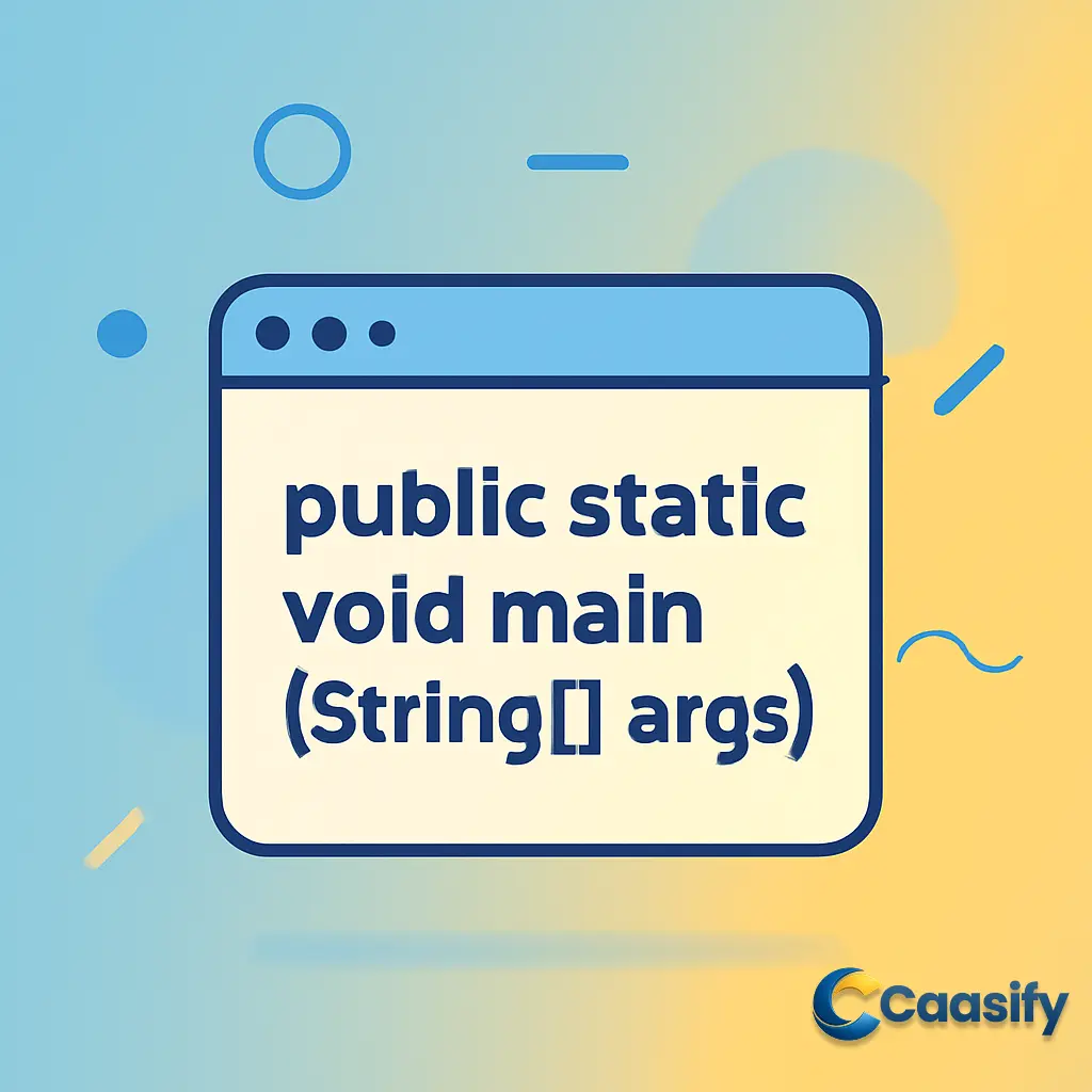
    The Java main method is a critical component for running standalone Java applications. Understanding the public static void main(String[] args) signature is essential for ensuring your program runs smoothly on the Java Virtual Machine (JVM). This method serves as the entry point, and its precise structure is crucial for execution. In this article, we’ll dive into the importance of the main method, how it interacts with the JVM, common errors developers face, and best practices for structuring and using the main method effectively. Whether you’re new to Java or looking to sharpen your skills, mastering the main method is key to building robust Java applications.

    What is Java main method?

    The Java main method is the essential entry point for running any standalone Java application. It is the method where the program starts, and it must follow a specific format: public static void main(String[] args). This method allows developers to pass command-line arguments and initiate the execution of the program. Without the correct signature, the Java Virtual Machine (JVM) cannot run the program.

    What Happens When the Main Method Signature is Altered?

    Let me tell you a story about why a very specific signature in Java is so important. It’s the signature that, if changed even a little, can stop your Java program from running altogether. We’re talking about the infamous public static void main(String[] args) – the main method. If anything in this signature is altered, the Java Virtual Machine (JVM) won’t recognize it as the starting point for your program, no matter how perfectly your code compiles.

    Imagine you’re about to launch your Java program, all excited and ready to see your code in action. But then, something goes wrong. Your program won’t run. The reason? The JVM has a very specific way of looking for that entry point. It doesn’t guess what you meant or search for similar methods. If it doesn’t find public static void main(String[] args), it won’t start. Let’s go over some of the things that can break this sacred signature.

    Missing the Public Modifier

    Picture this: You’ve written your main method, but for some reason, you decided to leave out the public modifier. Big mistake. Without it, the JVM won’t be able to find your main method from outside the class. You’ve essentially closed the door to the JVM, and it can’t get in. Here’s an example of what this looks like:

    public class Test {
    static void main(String[] args){
    System.out.println(“Hello, World!”);
    }
    }

    Now, you compile and run this code, thinking everything is fine. But here’s the error message you get instead:

    javac Test.java
    java Test
    Error: Main method not found in class Test, please define the main method as: public static void main(String[] args) or a JavaFX application class must extend javafx.application.Application

    So, what happened? Without the public modifier, the JVM just couldn’t see the method, and it refuses to start the program.

    Missing the Static Modifier

    Now, let’s imagine another scenario. You’ve missed the static keyword, thinking it’s not that important. But here’s the thing: The static keyword is crucial for the main method to work. When your Java program starts, the JVM loads the class but hasn’t created any objects yet. Without the static keyword, the main method is considered an instance method, meaning it needs an object to be called. But since no objects exist at the start, the JVM can’t invoke the main method.

    Take a look at this example:

    public class Test {
    public void main(String[] args){
    System.out.println(“Hello, World!”);
    }
    }

    If you compile and run this, you’ll see an error message like this:

    javac Test.java
    java Test
    Error: Main method is not static in class Test, please define the main method as: public static void main(String[] args)

    The JVM just doesn’t know what to do with it because it can’t find the static method. Without static, the program is stuck before it even begins.

    Changing the Void Return Type

    Java is very particular about the return type of the main method. It must be void—it doesn’t return anything. After all, the main method is the launchpad for the program, and once it finishes, the program ends. If you change that void to something like int, the JVM will get confused. You’ve basically redefined the method, and it will no longer be recognized as the main entry point.

    Take a look at this example where the return type is changed:

    public class Test {
    public static int main(String[] args){
    return 0;
    }
    }

    You might think this will work, but the JVM will throw an error when you compile:

    javac Test.java
    Test.java:5: error: incompatible types: unexpected return value
    return 0;
    ^
    1 error

    The JVM was expecting void, not an integer, so it can’t find the entry point. The program is stopped before it even starts.

    Altering the Method Name or Parameter Type

    The method name is the most sacred part of this process. It has to be main. The JVM is trained to search for a method called main, and if it doesn’t find it, well, your program just won’t run. You can’t just change the name to something like myMain—the JVM won’t recognize it. Even altering the parameter type from String[] args to something like String arg will mess things up.

    Here’s an example where the method name is changed:

    public class Test {
    public static void myMain(String[] args){
    System.out.println(“Hello, World!”);
    }
    }

    Compile and run this, and here’s the message you’ll get:

    javac Test.java
    java Test
    Error: Main method not found in class Test, please define the main method as: public static void main(String[] args) or a JavaFX application class must extend javafx.application.Application

    Now, you can see that the JVM simply didn’t find main, and without it, the program isn’t going anywhere.

    Similarly, changing the parameter type will have the same result. Take this example:

    public class Test {
    public static void main(String arg){
    System.out.println(“Hello, World!”);
    }
    }

    Here, you’ve changed the parameter from String[] args to String arg. This will confuse the JVM, and it won’t run your program. The JVM expects String[] args, and if you change it, the program’s entry point is lost.

    The Bottom Line: Keep That Signature Intact

    So, what’s the takeaway from all of this? It’s pretty simple: if you want your Java program to run, you have to stick to the exact signature for the main method. Don’t change the name, the return type, or the parameter. The JVM is picky, and if it doesn’t find the signature it expects, your program won’t run, no matter how perfect your code might be. So, remember: public static void main(String[] args) is your golden ticket to running Java programs. Stick with it, and your programs will run smoothly across any platform.

    Java SE Documentation: Java Main Method

    Why the Main Method Signature Must Be Exact

    Imagine you’re getting ready to run your favorite Java program. You’ve spent hours coding, testing, and perfecting every little detail. But here’s the catch – there’s a very specific way Java wants you to get things started. And no, it’s not just about writing any piece of code and calling it a day. The Java Virtual Machine (JVM) is very particular about the rules.

    When you run a Java program, the JVM follows a very strict protocol. It’s like a bouncer at a club who only lets in the people with the right invitation. And for Java, that invitation is the main method. The JVM knows exactly what to look for: it’s looking for the method signature public static void main(String[] args). No variations, no substitutions. If the JVM doesn’t find this exact signature, guess what? It’s not going to run your program.

    Now picture this: you’ve named your method “start” instead of “main” or maybe used a different return type, like “int” instead of “void.” The JVM won’t try to be creative. It won’t guess that your method is the one it should run. If it doesn’t find that precise signature, your program simply won’t launch. End of story.

    This requirement isn’t just a quirky Java thing; it’s built into how the language works. By sticking to this rigid signature, Java ensures that no matter where your program runs, it always knows where to start. Think of it as a map – the JVM knows exactly where to begin the journey, whether the program is running on Windows, Mac, or Linux.

    That’s the magic of Java’s portability. Thanks to this predictable entry point, Java can run seamlessly on just about any platform. Whether you’re developing an app for your laptop, your phone, or even a cloud-based server, Java’s consistency is a big reason it’s known as a versatile language. The JVM’s strict following of this method signature means that no matter the environment, Java programs always start in the same, reliable way.

    So, next time you’re writing that all-important public static void main(String[] args) method, remember: it’s not just about following the rules – it’s what keeps your Java program running smoothly on any platform, anywhere.

    Java Main Method Guidelines

    What Happens When the Main Method Signature is Altered?

    Let me tell you a story about the importance of a very specific signature in Java. It’s a signature that, if changed even a little, can stop your Java program from running at all. We’re talking about the infamous public static void main(String[] args) – the main method. If any part of this signature is changed, the Java Virtual Machine (JVM) won’t recognize it as the starting point for your program, no matter how perfectly your code compiles.

    Imagine you’re about to launch your Java program, full of confidence, ready to see your code in action. But then, something goes wrong. The program won’t run. The reason? The JVM has a very particular way of looking for that entry point. It doesn’t guess what you meant or search for similar methods. If it doesn’t find public static void main(String[] args), it won’t start.

    Let’s walk through some of the things that can break this sacred signature.

    Missing the Public Modifier

    Picture this: you’ve written your main method, but for some reason, you decided to leave out the public modifier. Big mistake. Without it, the JVM won’t be able to find your main method from outside the class. You’ve essentially closed the door to the JVM, and it can’t get in. Here’s an example of what this looks like:

    public class Test {
    static void main(String[] args){
    System.out.println(“Hello, World!”);
    }
    }

    Now, you compile and run this code, thinking everything is fine. But here’s the error message you get instead:

    Error: Main method not found in class Test, please define the `main` method as: public static void main(String[] args) or a JavaFX application class must extend javafx.application.Application

    So, what happened? Without the public modifier, the JVM just couldn’t see the method, and it refuses to start the program.

    Missing the Static Modifier

    Now, let’s imagine another scenario. You’ve missed the static keyword, thinking it’s not that important. But here’s the thing: the static keyword is crucial for the main method to work. When your Java program starts, the JVM loads the class but hasn’t created any objects yet. Without the static keyword, the main method is considered an instance method, meaning it needs an object to be called. But since no objects exist at the start, the JVM can’t invoke the main method.

    Take a look at this example:

    public class Test {
    public void main(String[] args){
    System.out.println(“Hello, World!”);
    }
    }

    If you try to compile and run this, you’ll see an error message like this:

    Error: Main method is not static in class Test, please define the `main` method as: public static void main(String[] args)

    The JVM just doesn’t know what to do with it because it can’t find the static method. Without static, the program is stuck before it even begins.

    Changing the Void Return Type

    Java is very particular about the return type of the main method. It must be void—it doesn’t return anything. After all, the main method is the launchpad for the program, and once it finishes, the program ends. If you change that void to something like int, the JVM will be confused. You’ve essentially redefined the method, and it will no longer be recognized as the main entry point.

    Take a look at this example where the return type is changed:

    public class Test {
    public static int main(String[] args){
    return 0;
    }
    }

    You might think this will work, but the JVM will throw an error when you compile:

    Test.java:5: error: incompatible types: unexpected return value
    return 0;
    ^
    1 error

    The JVM was expecting void, not an integer, so it can’t find the entry point. The program is stopped before it even starts.

    Altering the Method Name or Parameter Type

    The method name is the most sacred part of this process. It has to be main. The JVM is trained to search for a method called main, and if it doesn’t find it, well, your program just won’t run. You can’t just change the name to something like myMain—the JVM won’t recognize it. Even altering the parameter type from String[] args to something like String arg will mess things up.

    Here’s an example where the method name is changed:

    public class Test {
    public static void myMain(String[] args){
    System.out.println(“Hello, World!”);
    }
    }

    Compile and run this, and here’s the message you’ll get:

    Error: Main method not found in class Test, please define the `main` method as: public static void main(String[] args) or a JavaFX application class must extend javafx.application.Application

    Now, you can see that the JVM simply didn’t find main, and without it, the program isn’t going anywhere.

    Similarly, changing the parameter type will have the same result. Take this example:

    public class Test {
    public static void main(String arg){
    System.out.println(“Hello, World!”);
    }
    }

    Here, you’ve changed the parameter from String[] args to String arg. This will confuse the JVM, and it won’t run your program. The JVM expects String[] args, and if you change it, the program’s entry point is lost.

    The Bottom Line: Keep That Signature Intact

    So, what’s the takeaway from all of this? It’s pretty simple: if you want your Java program to run, you have to stick to the exact signature for the main method. Don’t change the name, the return type, or the parameter. The JVM is picky, and if it doesn’t find the signature it expects, your program won’t run, no matter how perfect your code might be. So, remember: public static void main(String[] args) is your golden ticket to running Java programs. Stick with it, and your programs will run smoothly across any platform.

    Java SE Documentation

    Variations in the Main Method Signature

    In the world of Java, there’s one method that stands above the rest—the infamous main method. It’s the method that kicks off every Java application, and it follows a strict signature. But here’s the thing: while the core structure of this method stays the same, there are a few areas where you can tweak it a bit without messing up your program. Knowing these small changes can make your code more readable, flexible, and reflect your personal coding style.

    The Parameter Name

    Let’s start with the parameter. Normally, you’ll see the String[] args as the standard. This is how the method accepts command-line arguments, which are the inputs you provide when you run the program. But here’s the cool part—you don’t have to stick with the name args! That’s just the conventional name, but you can change it to something that makes more sense for you. For instance, if your program is handling file paths, you might want to call it filePaths. You can name it anything that fits the context. Take a look at how that might look in your code:

    Standard Convention:

    public static void main(String[] args) {   // Standard ‘args’ parameter name }

    Valid Alternative:

    public static void main(String[] commandLineArgs) {   // The name has been changed, but the signature stays valid }

    It’s a small change, but it’s important to remember that the parameter must always be a String[] array. No matter what name you give it, the structure must remain the same because the JVM expects it.

    Parameter Syntax Variations

    Now, let’s explore some syntax variations. The String[] parameter in the main method can actually be written in a few different ways, and each variation is understood by the JVM. This gives you some freedom in how you write it. Let’s go through your options:

    Standard Array Syntax (Recommended): This is the classic and clean format where the brackets [] are placed after the type. It’s the most commonly used style because it’s clear and consistent.

    public static void main(String[] args) {   // Recommended syntax }

    Alternative Array Syntax: This syntax places the brackets after the parameter name. It’s more common in languages like C++, but it still works in Java. While it’s functional, it might seem a bit unusual to many Java developers.

    public static void main(String args[]) {   // Alternative syntax }

    Varargs (Variable Arguments): Introduced in Java 5, the varargs syntax lets you pass a variable number of arguments to the method. For the main method, this is functionally the same as String[] args, but it provides a bit more flexibility in some cases.

    public static void main(String… args) {   // Varargs syntax, equivalent to String[] args }

    While all three variations work perfectly fine, the String[] args syntax is the most widely used. It’s the Java convention and is recommended for consistency and clarity, especially in larger projects.

    The Order of Access Modifiers

    Now, let’s talk about the order of the access modifiers—public and static. These are both necessary for the JVM to find and run your main method. But here’s the twist: while they both need to be there, the order in which they appear doesn’t actually matter to the Java compiler. You could switch them around, and it will still work just fine. Let’s look at the standard order and an alternative one:

    Standard Convention:

    public static void main(String[] args) {   // Standard modifier order }

    Valid Alternative:

    static public void main(String[] args) {   // Alternative modifier order, still valid }

    Both orders are technically valid, but public static is the convention in Java. It’s considered best practice because it keeps your code clear and consistent, especially in larger projects or when working with teams. Following this convention improves the readability of your code and makes it easier for others (and even for you later on) to collaborate.

    Wrapping It All Up

    The flexibility in how you write the main method signature might seem like a small thing, but it actually gives you more freedom to express yourself in your code. You can rename the parameter to make it clearer, use a different syntax to suit your style, or change the order of modifiers if you prefer. As long as the core structure of public static void main(String[] args) stays the same, these little tweaks won’t affect how your program runs. So, go ahead, have fun tweaking it, but just make sure to keep it clear and consistent!

    For a detailed overview, visit the Java Main Method documentation at the official website.

    How to Use Command-Line Arguments in Java

    Alright, let’s talk about something that can really take Java programming from “just code” to “an awesome interactive experience”—command-line arguments. Sure, you’ve probably already got the basic idea of the public static void main(String[] args) method down, but the magic happens when you start using the String[] args parameter to bring in external data. This is where your program gets dynamic and responsive, picking up commands or data from the outside world—specifically, from the command line—every time you run it.

    Imagine this: you’re writing a program, and you want it to react to different users in a personalized way. You don’t want to hardcode their names into the program every time. Instead, you want it to take a name from the command line and greet them. That’s where args[] comes in. It’s like a little messenger, bringing in information that you can use while your program runs.

    Let’s see this in action. Here’s a simple, fun example: we’ll create a program that greets the user by name. When you run the program, you’ll pass in the name from the command line. The program then greets you as if you’re its best friend. Pretty cool, right?

    Here’s the code for the GreetUser program:

    public class GreetUser {
    public static void main(String[] args) {
    // The first argument is at index 0 of the ‘args’ array.
    String userName = args[0];
    System.out.println(“Hello, ” + userName + “! Welcome to the program.”);
    }
    }

    How It Works

    Step 1: Compile the Java Code

    First, you need to turn your Java program into something the JVM (Java Virtual Machine) can actually run. In other words, you need to compile it. You’ll do this by running the following command in your terminal or command prompt:

    $ javac GreetUser.java

    This creates a GreetUser.class file, which the JVM will be able to run.

    Step 2: Run the Program with Command-Line Arguments

    Next, let’s run the program. Here’s where the fun happens. Instead of just launching the program like usual, you’ll pass an argument from the command line. Let’s say you want the program to greet “Alice.” You’ll run the following command:

    $ java GreetUser Alice

    The Output

    Now, when you hit enter, the program takes the argument you passed (“Alice”) and sticks it in the args[0] position. It will then display a greeting message that’s personalized just for her:

    Hello, Alice! Welcome to the program.

    How the args[] Array Works

    In the background, what’s happening is that when you run $ java GreetUser Alice, the args[] array gets filled with the values you provided in the command line—so here, args[0] becomes “Alice.” You could add more arguments too. For example, you could pass a last name, a greeting, or even a custom message. The program simply grabs what’s passed and uses it.

    This simple example shows how you can use args[] to interact with your program dynamically, which is a pretty cool way to make the program feel more flexible based on user input. The value “Alice” that was passed in is used by the program to personalize the greeting message, making it feel a bit more human, don’t you think?

    More Possibilities

    And here’s the thing—this is just scratching the surface. You can extend this idea and allow your Java programs to accept multiple command-line arguments, offering even more flexibility in how the program behaves. You could make the program take in numbers, filenames, settings, or even configurations—whatever you need at runtime.

    So, by using command-line arguments in Java, you can add layers of interactivity and make your programs adaptable to different situations. Pretty powerful for such a simple tool, right? Whether you’re building small tools or larger applications, understanding how to make your program take user input via the command line is a real game changer!

    For further details, check out the official Java Command-Line Tutorial.

    Java Command-Line Tutorial

    Common Errors and Troubleshooting

    So, you’re diving into Java, huh? That’s awesome! But, as you might have already found out, it’s super easy to run into errors, especially with the famous main method. If you’re just starting, don’t worry, it happens to the best of us. You might type something wrong or miss a small detail, and boom, your program doesn’t work like you expected. But here’s the good news: these issues are usually pretty easy to fix once you know what to look for.

    In this guide, we’ll walk through the most common mistakes you’ll run into when working with the main method. I’ll explain what causes them, how to spot them, and how to fix them—so you can get back to coding with confidence.

    Error: Main Method Not Found in Class

    This one? It’s a classic. As a Java beginner, you’ll probably run into it sooner or later. Basically, the JVM is saying, “Hey, I can’t find the main method where I’m supposed to start.” The problem is that Java’s Virtual Machine (JVM) is super picky about the exact signature of the main method—if it’s even a little bit off, it won’t run.

    What does it look like? You might see an error message that says:

    Error: Main method not found in class YourClassName, please define the main method as: public static void main(String[] args)

    Common Causes:

    • A Typo in the Name: Maybe you accidentally typed maim instead of main. It happens!
    • Incorrect Capitalization: Remember, Java is case-sensitive. If you wrote Main instead of main, that’s enough to throw off the JVM.
    • Wrong Return Type: The main method must always have a void return type. If you put int or anything else, that’s a no-go.
    • Incorrect Parameter Type: The parameter must be String[] args. If you change it to something else, like main(String arg), it won’t work.

    How to Fix It:

    To solve this, double-check your main method and make sure it’s exactly like this:

    public static void main(String[] args)

    Error: Main Method is Not Static in Class

    This one’s a bit trickier, but still super common. When you try to run your program, the JVM might tell you it can’t invoke the main method because it’s not static. Now, you might be thinking, “Why does it have to be static?” Here’s the deal: when your program starts, no objects have been created yet. The JVM needs to call the main method directly from the class without creating an instance.

    What it looks like: You might see an error like this:

    Error: Main method is not static in class YourClassName, please define the main method as: public static void main(String[] args)

    Common Cause:

    You might have missed the static keyword in the method signature. Without it, the JVM can’t run your method because it doesn’t want to create an object first.

    How to Fix It:

    Just add the static keyword between public and void:

    public static void main(String[] args)

    This tells the JVM, “Hey, this method belongs to the class, not to any specific instance.”

    Runtime Error: ArrayIndexOutOfBoundsException

    This error doesn’t show up during compilation, but it’ll bite you once the program is running. It happens when you try to access an element in the args[] array that doesn’t exist.

    What it looks like: You might see an error like this:

    Exception in thread “main” java.lang.ArrayIndexOutOfBoundsException: Index 0 out of bounds for length 0 at YourClassName.main(YourClassName.java:5)

    Common Cause:

    This error usually happens if you try to access a command-line argument, like args[0], but the user hasn’t actually passed any arguments when running the program. In that case, args[0] doesn’t exist, and the program crashes.

    How to Fix It:

    Before you access any elements in the args[] array, always check the array’s length to make sure the arguments were provided. Here’s a quick fix:

    if (args.length > 0) {
    String userName = args[0];
    System.out.println(“Hello, ” + userName + “!”);
    } else {
    System.out.println(“No arguments provided.”);
    }

    This way, if the user forgets to provide input, the program won’t crash—it’ll just handle the situation gracefully.

    Compilation Error: Incompatible Types – Unexpected Return Value

    This is a compile-time error, which means it stops your program from running before it even gets the chance to. It happens when you try to return something from the main method.

    What it looks like: You might see something like this:

    YourClassName.java:5: error: incompatible types: unexpected return value
    return 0;
    ^
    1 error

    Common Cause:

    Remember, the main method has a void return type. That means it’s not supposed to return anything. If you try to return a value like return 0;, the compiler will throw an error.

    How to Fix It:

    Simply remove the return statement. If you need to indicate that the program ran successfully or had an error, use System.exit(0) to exit the program with a status code:

    public static void main(String[] args) {
    // Correct way to terminate with a status code
    System.exit(0);
    }

    By understanding these common errors and knowing how to troubleshoot them, you can avoid a lot of frustration. Each of these mistakes is a minor roadblock, but once you’ve got the hang of spotting them, debugging becomes way easier. So, the next time you see one of these errors, you’ll know exactly what to do to keep your Java programs running smoothly.

    Oracle Java Documentation

    Best Practices for the main Method

    Let me paint you a picture. You’ve just written your first Java program, and it’s looking pretty good. But now it’s time to scale up—add more features, handle more data, and make your program even better. As you start making your program more complex, you realize that your main method is quickly becoming a mess. It’s packed with logic, data parsing, and even calculations—all in one spot. You know it’s time to clean things up.

    Here’s the thing: the main method is your entry point into the program, like the front door to your house. It’s not the place to store all the heavy lifting. By keeping the main method lean and focused on its job—getting things started and passing the work along—you can make your code more maintainable, readable, and scalable.

    Keep the Main Method Lean

    Imagine if you tried to do everything in your living room. Sounds chaotic, right? Well, that’s what happens when the main method gets overloaded. The main method should act as a coordinator. Its job is to parse any command-line arguments and delegate tasks to other methods or classes. This keeps things clean and organized.

    Instead of packing all your logic into the main method, split it up into smaller, more manageable chunks. The main method becomes a simple, high-level entry point, while other methods or classes handle the heavy lifting. This makes your code easier to read, test, and maintain.

    For example, look at this neat solution:

    public class Main {
    public static void main(String[] args) {
    String userName = parseUserName(args);
    printGreeting(userName);
    } public static String parseUserName(String[] args) {
    // Logic for parsing user input
    return args[0];
    } public static void printGreeting(String userName) {
    // Logic for printing a greeting
    System.out.println(“Hello, ” + userName + “!”);
    }
    }

    In this version, the main method isn’t bogged down with parsing and printing. It just calls other methods to do the work. This keeps things tidy.

    Handle Command-Line Arguments Gracefully

    Alright, you’re ready to interact with the outside world. Command-line arguments are the way to go. They let you bring data into your program when you run it, making it much more flexible. But, and this is important, you need to handle these inputs carefully. Messing up the arguments could make your program crash. You don’t want that, right?

    Here’s how you handle it:

    • Check args.length: Before you even think about using those arguments, make sure they exist. If the user didn’t provide the required input, you need to deal with that gracefully.
    • Use try-catch blocks: When you’re parsing numbers or other sensitive data, you might run into errors like NumberFormatException or ArrayIndexOutOfBoundsException. A good ol’ try-catch block will catch those mistakes before they cause problems.

    Here’s an example:

    public class Main {
    public static void main(String[] args) {
    if (args.length == 0) {
    System.out.println(“No arguments provided.”);
    return;
    }
    try {
    int number = Integer.parseInt(args[0]);
    System.out.println(“You provided the number: ” + number);
    } catch (NumberFormatException e) {
    System.out.println(“Invalid number format: ” + args[0]);
    }
    }
    }

    Now, your program checks if the arguments are present and handles any errors before they crash the party. It’s a smooth operator.

    Use System.exit() for Clear Termination Status

    Sometimes, your Java program needs to let the outside world know how it did. Whether it was a success or failure, you need a way to indicate that. This is where System.exit() comes in.

    In scripting and automation, the outcome of your program can influence what happens next. By convention, you should use System.exit(0) to signal a successful run and System.exit(1) to signal an error. This exit code tells other systems what to expect.

    Here’s how it works:

    public class Main {
    public static void main(String[] args) {
    try {
    // Program logic here
    System.exit(0); // Indicating success
    } catch (Exception e) {
    System.exit(1); // Indicating error
    }
    }
    }

    Think of System.exit() as the “Goodbye!” at the end of your program. It ensures that any automated systems or scripts know exactly what happened.

    Use a Dedicated Entry-Point Class

    If your program is simple, it’s fine to put everything in one class. But what happens when your project starts growing? More methods, more logic, more files. Keeping everything in one place makes things chaotic and hard to manage.

    That’s when you need a dedicated entry-point class—something like Application.java or Main.java. This class does one thing: starts the program. Everything else gets handled by other classes. This separation helps you keep your project neat and organized as it grows.

    For example:

    public class Main {
    public static void main(String[] args) {
    Application app = new Application();
    app.start();
    }
    }class Application {
    public void start() {
    // Core logic for the application
    System.out.println(“Application has started.”);
    }
    }

    By having a dedicated class for the entry point, you give your program a clean structure that’s easy to navigate—especially as your project scales.

    By following these best practices, you’ll not only write cleaner, more readable code, but you’ll also set yourself up for success as your Java programs grow. These tips help you keep things flexible, organized, and easy to maintain, no matter how complex your project gets. Plus, they’ll make your code easier to troubleshoot and extend as new features come along.

    For more detailed Java coding conventions, refer to the official Java Code Conventions (Oracle).

    Frequently Asked Questions (FAQs)

    So, you’re diving into the world of Java, and you’ve probably come across the famous method that every Java program starts with: public static void main(String[] args). But what does all this really mean? Let’s break it down together, step by step, so you can see exactly why this method is so crucial for running Java applications.

    What does public static void main mean in Java?

    When you’re starting a Java application, the Java Virtual Machine (JVM) looks for a very specific entry point to kick things off. That’s where the main method comes in. It’s the method that the JVM is programmed to search for and execute first when you run your program.

    Now, let’s take a closer look at each keyword in public static void main(String[] args) to see why it’s so important:

    • public: This is an access modifier, and it ensures that the method is accessible from outside the class. Since the JVM is an external process, it needs access to the main method to launch your program.
    • static: The static keyword means that the method belongs to the class itself, not to any instance (or object) of the class. This is key because when the JVM launches your program, there are no objects yet created, so it needs a method that can be called without any objects.
    • void: This tells the JVM that the main method doesn’t return anything. The sole purpose of the main method is to start the program; it doesn’t need to give any value back to the JVM after it’s done.
    • main: This is the name of the method, and it’s non-negotiable. The JVM is specifically looking for a method named main (with a lowercase “m”), and if it doesn’t find it, your program won’t run.
    • (String[] args): These are the command-line arguments passed to your program. The String[] part means that this method expects an array of strings. You can pass input like filenames, configuration settings, or other data through this array when launching the program.

    Let’s see the main method in action with a simple “Hello, World!” program:

    public class MyFirstProgram {
    // This is the main entry point that the JVM will call.
    public static void main(String[] args) {
    System.out.println(“Hello, World!”);
    }
    }

    In this basic example, the JVM looks for the main method, starts the program, and prints “Hello, World!” to the console.

    Why is the main method static in Java?

    Ah, the static keyword—this one’s a biggie! You might be wondering, “Why can’t the JVM just call an instance method to start things off?” Well, here’s the thing: when your program starts, no objects exist yet. The JVM loads the class into memory, but no instance of the class is created. Since instance methods need an object to be called upon, this would cause a problem.

    That’s why the main method needs to be static—it allows the JVM to call it directly from the class without needing to create an object first. The static keyword makes the main method independent of any object, so it can be the starting point for the JVM.

    What is the purpose of String[] args?

    Now, let’s talk about that String[] args parameter. This is where the magic happens. The args array allows your Java program to accept command-line arguments. This means, you can pass information from the command line directly into your program when it starts. Cool, right?

    For example, if you run your program like this:

    $ java MyProgram “John Doe” 99

    The args array will contain the following:

    args[0] = “John Doe”
    args[1] = “99”

    Now you can use those values inside your program. Check out how you can greet the user with their name:

    public class MyProgram {
    public static void main(String[] args) {
    if (args.length > 0) {
    System.out.println(“Hello, ” + args[0]); // Prints: Hello, John Doe
    } else {
    System.out.println(“Hello, stranger.”);
    }
    }
    }

    With the command above, the program will print “Hello, John Doe!” or “Hello, stranger.” depending on whether or not the user provided input.

    What happens if a Java program doesn’t have a main method?

    Picture this: you’ve written your Java program, but when you try to run it, nothing happens. The reason? If the program doesn’t include that exact public static void main(String[] args) signature, it will compile just fine, but the JVM won’t know where to start. When you try to run the program, the JVM will throw a NoSuchMethodError.

    You might see something like this:

    Error: Main method not found in class MyProgram, please define the main method as:
    public static void main(String[] args)

    Without the main method, your program has no entry point, and the JVM can’t launch it. Simple as that.

    Can a Java class have more than one main method?

    Here’s a fun fact: yes, a Java class can have more than one method named main, as long as their parameters are different. This is called method overloading. However, the JVM only recognizes the method with the exact signature public static void main(String[] args) as the program’s entry point. Any other main methods are just regular methods—nothing special.

    Check this out:

    public class MultipleMains {
    // This is the only method the JVM will execute to start the program.
    public static void main(String[] args) {
    System.out.println(“This is the real entry point.”);
    // We can call our other ‘main’ methods from here.
    main(5);
    } // This is an overloaded method. It is not an entry point.
    public static void main(int number) {
    System.out.println(“This is the overloaded main method with number: ” + number);
    }
    }

    In the example above, only the main(String[] args) method will be called by the JVM to start the program. The other method can be called inside it, but it’s not the entry point.

    Can I change the signature of the main method?

    Now, you might be thinking, “Can I change the main method to suit my needs?” Well, sort of! While there are a few small tweaks you can make, the core parts of the method signature can’t be changed. Here’s what you can and can’t modify:

    What You CAN Change:

    • The parameter name: You can rename args to something else, like myParams or inputs.
    • The array syntax: You can use a C-style array declaration like String args[].
    • Varargs: You can use the varargs syntax introduced in Java 5: String… args.
    • Modifier order: You can swap the order of public and static, like static public void main(…).

    What You CANNOT Change:

    • public: It can’t be private, protected, or have no modifier.
    • static: It can’t be a non-static instance method.
    • void: It must not return a value.
    • main: The method name must be exactly main. “Main” with an uppercase “M” won’t work.

    Why is the main method public and not private?

    Ah, this one’s easy. The main method must be public because it needs to be visible to the JVM. In Java, access modifiers like public and private control who can see and access a method. If the main method were private, it would only be accessible within the same class, which is a problem because the JVM is an external process. The public modifier ensures the JVM can see and execute the method to start the program.

    So, there you have it—the inner workings of the main method in Java. You might have a few more questions down the line, but now you’re equipped to understand why this little method is so crucial to your Java applications.

    What is the main method in Java?

    Conclusion

    In conclusion, understanding the Java main method is crucial for any developer working with Java applications. This method serves as the starting point for your program, ensuring that the Java Virtual Machine (JVM) can execute it correctly. We’ve explored the essential components of the public static void main(String[] args) signature, why the syntax is so strict, and how variations can impact your program’s functionality. Additionally, we discussed common errors and best practices for structuring your main method and working with command-line arguments, which will help make your code more maintainable and flexible.As Java continues to evolve, staying updated on the latest practices related to the main method and JVM can improve the efficiency and scalability of your applications. So, whether you’re a beginner or an experienced developer, mastering the main method is key to writing successful Java programs.With the understanding of Java’s main method and JVM interaction, you can now write cleaner, more efficient code. Keep refining your skills and adapt to new Java trends to stay ahead in the development world.

  • Master Python Script Execution on Ubuntu with Python3 and Virtual Environments

    Master Python Script Execution on Ubuntu with Python3 and Virtual Environments

    Introduction

    Running Python scripts on Ubuntu requires more than just typing out commands—it’s about managing dependencies, ensuring compatibility, and optimizing your development environment. With Python 3 and virtual environments, you can streamline your workflow and avoid conflicts between different versions of Python. This article will guide you through setting up Python 3, creating scripts, managing packages, and troubleshooting common errors on Ubuntu. Whether you’re working with legacy systems or building new applications, understanding how to leverage virtual environments will help you maintain a clean, efficient development setup. Let’s dive into the process and master Python script execution on Ubuntu!

    What is Virtual environments?

    Virtual environments are isolated spaces where you can store the specific libraries and versions needed for a Python project. This helps prevent conflicts between different projects by keeping their dependencies separate, making it easier to manage multiple projects with different requirements.

    Step 1 – How to Set Up Your Python Environment

    So, you’ve got Ubuntu 24.04 up and running, and here’s the good news—it already comes with Python 3 installed by default! This means you usually won’t have to install it manually unless you’re dealing with something a bit special. But still, it’s always a good idea to make sure that Python 3 is properly set up on your system.

    To do that, just open your terminal and type in this simple command:

    $ python3 –version

    When you run it, your terminal will show you something like “Python 3.x.x,” where the “x.x” represents the exact version of Python 3 that’s installed. If you see that, you’re all set! Python 3 is already there, ready for action.

    But what if you don’t see that? Or maybe you get an error saying something like “command not found”? No worries—that just means Python 3 isn’t installed yet, but that’s not a big deal at all. All you need to do is install it with this command:

    $ sudo apt install python3

    This command will grab the latest version of Python 3 from Ubuntu’s software repository. It’ll only take a minute, and once it’s done, just run python3 –version again. You should see that Python 3 is now installed and ready to go!

    Next up: pip. If you’re going to be working with Python (and let’s be honest, you probably will), you’ll need pip. It’s the tool that helps you easily manage Python libraries and packages. You’ll be using it to install things like numpy, scikit-learn, and anything else your project needs. To install pip, just run:

    $ sudo apt install python3-pip

    Once pip is installed, you’ll be able to use it to easily download and manage Python packages. Now you’re all set! Your Python 3 environment on Ubuntu is good to go, and you’re ready to start coding.

    For more details, check out the Ubuntu Python 3 Installation Guide.

    Step 2 – How to Create Python Script

    Alright, now that we’ve got everything set up, it’s time to get our hands dirty and start writing some Python code! This is where the fun really begins. First, you’ll want to head to the folder where you want to save your script. Think of this like picking the spot on your computer where you’re going to keep all your important files. To do that, simply run this command in the terminal:

    $ cd ~/path-to-your-script-directory

    Once you’re in the right place, it’s time to create a Python script. But how do you actually make a new script? Don’t worry, it’s simple—we’re going to use the nano text editor. It’s super easy to use. Just type this command in the terminal:

    $ nano demo_ai.py

    This will open up the nano editor, giving you a fresh blank text file to work with. Now you’re all set to write your Python code. You can either write your own from scratch or copy the example I’m about to show you. Here’s a simple script to get you started:

    from sklearn.tree import DecisionTreeClassifier
    import numpy as np
    import random

    # Generate sample data
    x = np.array([[i] for i in range(1, 21)])    # Numbers 1 to 20
    y = np.array([i % 2 for i in range(1, 21)])    # 0 for even, 1 for odd

    # Create and train the model
    model = DecisionTreeClassifier()
    model.fit(x, y)

    # Function to predict if a number is odd or even
    def predict_odd_even(number):
        prediction = model.predict([[number]])
        return "Odd" if prediction[0] == 1 else "Even"

    if __name__ == "__main__":
        num = random.randint(0, 20)
        result = predict_odd_even(num)
        print(f"The number {num} is an {result} number.")

    At first glance, this might look a bit complicated, but let me walk you through it. The purpose of this script is pretty simple: it predicts whether a number is odd or even. But how does it do that? Well, it uses something called a DecisionTreeClassifier from the scikit-learn library—a tool that helps the script “learn” from data. Here’s what’s going on in the script:

    • Data Generation: x is a list of numbers from 1 to 20. We’ll use these numbers as input for our machine learning model. y contains labels for each number: 0 for even numbers and 1 for odd numbers. So, for example, the number 2 gets labeled with a 0 (because it’s even), and the number 3 gets labeled with a 1 (because it’s odd).
    • Model Creation and Training: We create a DecisionTreeClassifier and train it using the x and y data. This helps the model figure out how to predict whether a number is odd or even.
    • Prediction Function: The predict_odd_even(number) function takes a number as input and uses the trained model to predict whether that number is odd or even. It uses the model.predict() method to make that prediction.
    • Random Number Generation: In the __main__ part of the script, we generate a random number between 0 and 20 using random.randint(0, 20). This is where the magic happens! The script then predicts whether that number is odd or even and prints the result.

    Running the Script: Once you’ve written your code, don’t forget to save it! In nano, press CTRL + X, then hit Y to confirm saving, and finally, hit Enter to exit the editor.

    This script is a basic example of how you can use machine learning in Python to classify data. It’s not just about simple math—it’s about teaching a model to spot patterns, like figuring out whether a number is odd or even. And the best part? You can take this idea and apply it to much more complex problems down the road!

    Scikit-learn: Classifier Comparison

    Step 3 – How to Install Required Packages

    Alright, now we’re getting into the fun part—installing the packages that will bring your script to life! One of the most important packages you’ll need is NumPy. It’s a powerful library that’s super useful when it comes to creating and working with datasets. In the script we worked on earlier, NumPy was used to generate the dataset for training the machine learning model. Without it, things would get a bit tricky!

    Here’s the deal: starting with Python 3.11 and pip version 22.3, there’s a change in how Python environments are handled. It’s called PEP 668, and it introduces the idea of marking Python base environments as “externally managed.” What does that mean for you? Well, if you try to install packages using pip3 in certain environments, you might run into an error like “externally-managed-environment.” For example, if you run this command:

    $ pip3 install scikit-learn numpy

    You’ll get an error instead of the expected result. Frustrating, right? But don’t worry, there’s a fix!

    To get around this, you’ll need to create a virtual environment. Think of it as your own little isolated space where you can install Python packages without messing with the system-wide Python setup. It’s like having your own personal workspace, where you can keep things neat without affecting anyone else’s work.

    Let’s walk through how to set up that virtual environment:

    Installing virtualenv

    First, you need to install virtualenv, which is the tool that lets you create and manage these isolated environments. To install it, run this simple command:

    $ sudo apt install python3-venv

    Once that’s done, you’re all set to create a virtual environment in your project directory.

    Creating the Virtual Environment

    To create your environment, run this command:

    $ python3 -m venv python-env

    This will create a new directory called python-env in your current directory. Inside this folder, you’ll have a fresh Python environment—clean, neat, and ready to go.

    Activating the Virtual Environment

    Next, let’s get that environment activated so it can start doing its thing. Run this command:

    $ source python-env/bin/activate

    Once you do that, something cool happens: your terminal prompt will change. You’ll see the name of your virtual environment in parentheses, like this:

    (python-env) ubuntu@user:~

    This is your visual cue that you’re now working within your isolated environment. From here on out, any packages you install or commands you run will stay separate from the system Python setup. You’re in your own little world now—perfect for managing dependencies and avoiding conflicts.

    Installing the Required Packages

    Now that your environment is up and running, let’s get those packages installed! To install scikit-learn and NumPy, which are crucial for machine learning tasks, run:

    $ pip install scikit-learn numpy

    scikit-learn is essential for data mining, machine learning, and data analysis. It’s a must-have for any data science project.

    NumPy helps with handling arrays and numerical data, making complex calculations and data manipulations a breeze.

    And here’s a little bonus: You don’t even need to install the random module. It’s already part of Python’s standard library, so it’s good to go by default.

    Why Is This Important?

    Setting up a virtual environment and installing the required packages this way is a best practice in Python development. It ensures your environment stays isolated, so it doesn’t mess with other projects you’re working on. Plus, it’s super helpful when you need different versions of packages or Python for other projects. This approach keeps everything organized, clean, and hassle-free.

    By following these steps, you’ve successfully set up your own isolated Python environment, installed all the packages you need, and ensured everything is running smoothly. Now you’re all set to dive into your project with a clean and well-managed workspace!

    For a more detailed explanation on Python Virtual Environments, check out the full guide here.

    Step 4 – How to Run Python Script

    Alright, you’ve done the tough part—setting up your virtual environment and installing all the packages you need. Now it’s time for the fun part: running your Python script and seeing everything come to life!

    To start, head over to the folder where you’ve saved your Python script. If you’re not quite sure where that is, just use the terminal to navigate there. Once you’re in the right place, you’re all set to run the script. All you have to do is type this command:

    $ python3 demo_ai.py

    This command tells your Ubuntu system to run the script using Python 3. If everything’s set up correctly, the script will run, and you’ll see the output right in your terminal. It’s like flipping a switch and watching everything work!

    For example, when you run the script, you might see something like this:

    (python-env) ubuntu@user:~/scripts/python demo_ai.py
    The number 5 is an Odd number.

    In this case, the script randomly picked the number 5, and based on the machine learning model you trained earlier, it correctly predicted that 5 is an odd number. Cool, right?

    Now, here’s where it gets even cooler. If you run the script again, you’ll probably get a different result. For example:

    (python-env) ubuntu@user:~/scripts/python demo_ai.py
    The number 17 is an Odd number.

    This shows off the randomness in action! The random.randint() function is generating a new number each time the script runs, and then it gets classified as either odd or even based on the decision tree model you created.

    This isn’t just about seeing the same thing again and again—it’s about your script using a trained machine learning model to make predictions. Every time you run it, you get a fresh random number, and the model figures out whether it’s odd or even. Pretty cool, right?

    By following these steps, you’ve successfully run your first Python 3 script, brought machine learning to life, and seen how your model classifies numbers. This is the magic of using virtual environments and Python—everything is isolated, clean, and ready for more advanced tasks!

    For more information on Python basics, check out the Beginner Python Tutorials.

    Step 5 – How to Make the Script Executable [OPTIONAL]

    Alright, you’ve done all the hard work—your script is set up, your virtual environment is running smoothly, and Python 3 is installed. But here’s the thing: you can make your Python script even more efficient by making it executable. It’s totally optional, but trust me, it’s a cool little hack that saves you time and effort.

    Once your script is executable, you won’t have to type python3 demo_ai.py every time you want to run it. Instead, you can just run the script directly from the terminal, just like any other command. Pretty awesome, right? Let’s walk through how to do it.

    Open the Python Script

    First, you’ll need to open your Python script in a text editor. You can use the nano text editor for this. Just run the following command in your terminal:

    $ nano demo_ai.py

    This opens up the script in nano, where you can make changes.

    Add the Shebang Line

    Here’s the magic step: at the very top of your script, you need to add a shebang line. This is a special line that tells your operating system which interpreter to use when running the script. Since we’re using Python 3, you’ll need to add this line as the very first thing in the file:

    #!/usr/bin/env python3

    This tells the system, “Hey, use Python 3 to run this script,” no matter where Python 3 is installed on your machine.

    Save and Close the File

    Once you’ve added the shebang line, it’s time to save your work. In nano, do this by pressing CTRL + X to exit the editor. Then, press Y to confirm that you want to save the changes, and hit Enter to finalize it. Boom, your file is saved!

    Make the Script Executable

    Now for the fun part: making your script executable. This step is all about changing the file’s permissions so it can be run directly. To do that, run this command in your terminal:

    $ chmod +x demo_ai.py

    What this does is grant your script execute permissions, meaning it’s now ready to run just like any other command in your terminal.

    Run the Script Directly

    Now that your script is executable, you can skip the python3 part entirely. Instead of typing:

    $ python3 demo_ai.py

    You can simply run the script like this:

    ./demo_ai.py

    That’s it! When you run this command, your script will execute, and you should see the same output as before. The Python 3 interpreter will still be used, thanks to the shebang line you added.

    Why Bother?

    By making your script executable, you’ve just streamlined the process. It’s a small change that saves you from typing python3 every time you run the script. It’s quicker, easier, and just feels more natural when working with your Python scripts. Plus, it’s one of those little touches that make coding feel more like a smooth, efficient workflow.

    So, now you’ve got a Python script that runs with just a single command. It’s one more step toward making your development process faster and more convenient—just the way we like it!

    How to Make a Python Script Executable on Linux

    How to Handle Both Python 2 and Python 3 Environments

    Imagine you’re juggling two different versions of Python—one foot in the past, the other in the future. That’s what it’s like managing both Python 2 and Python 3 on your Ubuntu system. It’s like trying to fit two different puzzle pieces into the same frame. But, don’t worry, you can totally make it work.

    The key to managing these two Python versions is simple: use clear commands when running scripts and set up virtual environments for your projects. This way, you stop the versions from stepping on each other’s toes. No more conflicts between packages and dependencies. By isolating each project in its own virtual environment, you can easily switch between Python versions without worrying about them interfering with each other.

    Before we dive deeper into the setup, here’s something important to keep in mind: Python 2 is officially obsolete. It hasn’t received any updates since 2020, and it’s no longer supported. No security patches, no bug fixes—it’s like an old car that you keep driving around but isn’t really safe anymore. For any new projects, you definitely want to use Python 3 and virtual environments (venv). You can reserve Python 2 only for those old, legacy projects that still need it.

    How to Identify System Interpreters

    Now, let’s see what’s on your system. To check if you’ve got both Python 2 and Python 3 installed, you can easily check by running a couple of commands in the terminal.

    First, check for Python 3 by typing:

    $ python3 –version

    This will show you the version of Python 3 installed on your system. If it’s installed, you should see something like Python 3.x.x (where “x” represents the version number).

    Then, check for Python 2 by running:

    $ python2 –version

    If the terminal responds with something like “command not found,” it means Python 2 isn’t on your system anymore or it’s been removed. In that case, you’re only working with Python 3, and you can just focus on that.

    How to Explicitly Run Scripts

    Now that you know what versions of Python are available, it’s time to get to the fun part—running your scripts! The trick to making sure your script runs with the right version is to be clear about which one you’re using.

    If you want to run a script with Python 3, just type:

    $ python3 your_script_name.py

    If, for some reason, you’re still working with Python 2, use:

    $ python2 your_script_name.py

    This way, there’s no confusion. Your system knows exactly which version to use, and you won’t run into compatibility issues. Simple, right?

    How to Manage Projects with Virtual Environments (Best Practice)

    Here’s the best way to handle your projects, especially if you’re switching between Python 2 and Python 3: use virtual environments. These are isolated spaces where you can store project-specific dependencies, separate from the global Python setup. This approach solves what developers call “dependency hell,” where projects need different versions of the same package and everything gets messy.

    By using virtual environments, you can create separate, neat workspaces for each project, making sure that each one has the right dependencies—without any clashes.

    How to Create a Python 3 Environment with venv

    Creating a virtual environment with Python 3 is super easy, and the best part is that venv, the tool to create them, comes pre-installed with Python 3. But just in case it’s missing, here’s how you can get it:

    First, you might need to install venv with the following commands:

    $ sudo apt update
    $ sudo apt install python3-venv

    Once you’ve got that, let’s make your environment. To create a new virtual environment, just run:

    $ python3 -m venv my-project-env

    This will create a new directory called my-project-env, where all the magic happens. It’s like setting up a clean, isolated workspace for your project.

    To get started with your environment, activate it by running:

    $ source my-project-env/bin/activate

    After you do this, you’ll notice that your terminal prompt changes. It will now show something like:

    (my-project-env) ubuntu@user:~

    This means you’re working within your virtual environment, and any Python or pip commands you run will only affect this project. Super neat, right?

    How to Create a Python 2 Environment with virtualenv

    If you’re dealing with a legacy project that requires Python 2, you’ll need the virtualenv package. This is just like venv for Python 3, but it’s made to work with Python 2.

    Here’s how to set it up:

    First, make sure you’ve got virtualenv, Python 2, and pip installed by running:

    $ sudo apt install python3 python3-pip virtualenv

    If you’re on Ubuntu 20.04 or later, you might need to enable the universe repository or manually download Python 2 if it’s not available through your package manager.

    To create the Python 2 virtual environment, use this command:

    $ virtualenv -p /usr/bin/python2 my-legacy-env

    Once that’s done, activate your environment like this:

    $ source my-legacy-env/bin/activate

    Now, you’re inside your Python 2 virtual environment. The terminal prompt will let you know, and any Python commands will be executed with Python 2. If you’re done, just run:

    $ deactivate

    This will take you back to your global Python environment.

    Understanding Shebang Lines

    A shebang line is the first line in a script that tells the operating system which interpreter to use. Think of it like giving your computer a map to figure out how to run your script.

    For Python 3, the shebang line should look like this:

    #!/usr/bin/env python3

    And for Python 2, it would be:

    #!/usr/bin/env python2

    Once you’ve added the appropriate shebang line, you need to make the script executable. This is done by changing the file permissions with:

    $ chmod +x your_script.py

    Now, instead of typing python3 your_script.py every time, you can simply run the script directly:

    $ ./your_script.py

    If you want to run your script from anywhere, move it to a directory in your system’s PATH, like /usr/local/bin. That way, you can execute it without being in the same folder.

    With virtual environments, multiple Python versions, and shebang lines, you can keep your projects organized, avoid compatibility issues, and have everything running smoothly. It’s a bit of setup, but once it’s done, your workflow will be a lot more efficient!

    Python Virtual Environments: A Primer

    How to Identify System Interpreters

    So, you’re diving into Python on your Ubuntu system, but you need to figure out which versions of Python are installed, right? Don’t worry, it’s pretty simple! Think of it like checking which tools you’ve got—are you working with the shiny, modern Python 3, or do you still have some Python 2 hanging around? Here’s how you can check and know for sure.

    Checking for Python 3

    The first thing you’ll want to do is confirm if Python 3 is installed. Luckily, it’s really easy to check. Just open your terminal and type:

    $ python3 –version

    If Python 3 is installed, you’ll see something like Python 3.x.x (where “x.x” represents the version number). For example, it might say Python 3.8.5, or whatever version you have. That’s your confirmation that Python 3 is good to go!

    Checking for Python 2

    Now, let’s check for Python 2. If you’re working with older projects, you might still need this version. To see if it’s installed, run:

    $ python2 –version

    If Python 2 is around, this command will show you the version number, like Python 2.7.18. However, if Python 2 isn’t installed, you’ll get a “command not found” message, which means it’s not there anymore.

    What Does This All Mean?

    Here’s where it gets important. If you run the python2 command and get an error, that means Python 2 is gone, and Python 3 is probably your only option. And honestly, that’s becoming the standard these days. Since Python 2 reached its end of life in 2020, it’s no longer getting updates or security patches. It’s like keeping an old smartphone that doesn’t support new apps anymore. So, if you’re starting new projects, Python 3 is the way to go.

    By running these commands, you’ll quickly figure out what you’ve got on your system. It’s like checking your toolkit before you get to work—once you know what’s available, you can be sure you’re using the right Python version for your project.

    For more information, you can refer to the Install Python 3 on Ubuntu tutorial.

    How to Explicitly Run Scripts

    Alright, so you’ve got your Python script ready to go, but there’s one thing you need to make sure of: you’re running it with the right version of Python. It might seem like all you have to do is type python your_script.py, but here’s the thing—if you’ve got both Python 2 and Python 3 on your Ubuntu system, the default command might not always point to the version you expect. That’s where being specific comes in. You can take control and make sure the right interpreter runs your script. Let’s break it down!

    Running a Script with Python 3

    To run your script using Python 3, all you have to do is tell your terminal exactly what you want by typing:

    $ python3 your_script_name.py

    Now, this is super important: always use python3 instead of just python. On many systems, python might still point to Python 2, especially if both versions are installed. Using python3 ensures that Python 3 is running the script, so you won’t run into any unexpected issues. It’s like telling your computer, “Hey, I’m using Python 3—no surprises!”

    Running a Script with Python 2

    But what if you need to run your script with Python 2? Maybe you’re maintaining an old project that still relies on Python 2. Even though Python 2 is now outdated, you can still make it work with a simple command:

    $ python2 your_script_name.py

    This command will run your script with Python 2—if it’s installed, of course. Just keep in mind, Python 2 isn’t officially supported anymore. So, you’re really only using it if you absolutely have to, like with legacy projects that can’t be upgraded. For anything new, Python 3 should be your go-to.

    Why Being Explicit Matters

    By explicitly specifying which version of Python to use, you’re making sure your script runs smoothly every time. This method helps you avoid any potential conflicts, making sure you don’t run into version mismatches. After all, you don’t want to be left wondering why your script behaves differently depending on the environment, right?

    So, by controlling which version runs your code, you can keep things clean, predictable, and ready for anything!

    Always ensure you’re using the correct version for consistency and compatibility across systems.

    Python Version Documentation

    How to Manage Projects with Virtual Environments (Best Practice)

    Imagine you’re juggling multiple Python projects—one project needs a specific version of Python, while another might require completely different libraries or even a different version of Python. Without a clear structure in place, things can get messy really fast. This is where virtual environments come to the rescue.

    A virtual environment is like creating a separate, self-contained world where you can set up exactly what you need for a project, without it interfering with other projects or the global Python setup on your Ubuntu system. Think of it as having different rooms for each of your projects, each one with its own set of tools and resources. This way, you avoid “dependency hell,” which happens when two projects need different versions of the same library, and everything starts falling apart. Virtual environments make sure everything stays neatly organized, so each project can thrive without stepping on the toes of another.

    How to Create a Python 3 Environment with venv

    The venv module is built right into Python 3, and it’s the easiest and best way to create these isolated environments. It’s simple to use and ensures your projects stay organized. Let’s walk through the steps!

    Install venv (if needed) If you don’t already have venv installed, don’t worry—it’s really easy to set up on Ubuntu. Just open up your terminal and run these commands to get venv ready:

    $ sudo apt update
    $ sudo apt install python3-venv

    This will install venv on your system.

    Create the Virtual Environment Once venv is installed, creating a virtual environment is really easy. In your terminal, run:

    $ python3 -m venv my-project-env

    This command will create a new folder called my-project-env in your current directory. Inside this folder, you’ll find a fresh Python 3 interpreter and all the libraries you need for your project—completely separate from anything else on your system. Think of it as setting up a clean workspace just for this project.

    Activate the Virtual Environment Now for the fun part! To start using your virtual environment, you need to activate it. Run this command:

    $ source my-project-env/bin/activate

    Once activated, you’ll notice your terminal prompt changes to show the name of your virtual environment, like this:

    (my-project-env) ubuntu@user:~/your-project-directory$

    This means you’re working within your virtual environment, and any Python or pip commands you run will now use the Python 3 interpreter inside the my-project-env environment. You’re all set to start working on your project, without worrying about messing with other environments.

    How to Create a Python 3 Environment with virtualenv

    If you’re working on a legacy project or just want more flexibility, you might want to use virtualenv instead of venv. virtualenv is a third-party tool that gives you extra features, especially when you need to manage Python 2 environments. Here’s how to set it up:

    Install Prerequisites Before you can use virtualenv, make sure Python 3, pip, and the virtualenv package are installed. Run these commands:

    $ sudo apt install python3 python3-pip virtualenv

    If you’re using Ubuntu 20.04 or later, you might need to enable the universe repository or manually download Python 2 if it’s not available via the package manager.

    Create the Virtual Environment with Python 2 If you’re maintaining an old project that needs Python 2, you can still use virtualenv to create a Python 2 environment. Run this command:

    $ virtualenv -p /usr/bin/python2 my-legacy-env

    This will create a virtual environment called my-legacy-env that uses Python 2 as its interpreter. Cool, right?

    Activate the Virtual Environment Once your environment is set up, you’ll need to activate it:

    $ source my-legacy-env/bin/activate

    Now, when you look at your terminal prompt, you’ll see the environment name, like this:

    (my-legacy-env) ubuntu@user:~/your-project-directory$

    This means you’re working inside your Python 2 virtual environment. All your python and pip commands will now use Python 2.

    Deactivate the Virtual Environment When you’re done with your project and want to leave the virtual environment, you can deactivate it by typing:

    $ deactivate

    This will take you back to your system’s default Python environment.

    Wrapping It All Up

    Whether you’re using venv for Python 3 or virtualenv for legacy Python 2, virtual environments are a game changer. They let you keep your projects isolated, ensure your dependencies are clean, and make sure you’re always using the right version of Python. This practice saves you time, helps avoid frustration, and keeps everything running smoothly while juggling multiple projects. You’ll never have to worry about breaking things again, as long as you’re working within your own, neat environment!

    Python Virtual Environments: A Primer

    How to Create a Python 3 Environment with venv

    Imagine you’re juggling multiple Python projects on your Ubuntu system. One project needs a specific version of a library, while another requires something completely different. Without a solid plan in place, these conflicting dependencies could cause all sorts of issues with your workflow, right? That’s where venv comes to the rescue. The venv module, built right into Python 3, is the key to creating these isolated project environments. Think of it as a separate workspace for each of your projects. You can experiment safely, install different versions of libraries, and work on multiple projects without worrying about them interfering with each other or the global Python environment on your Ubuntu system. Let’s walk through how to get it set up.

    Install venv (if needed)

    In most cases, venv is already installed with Python 3, so you’re good to go. But just in case it’s not there, it’s easy to install. First, make sure your system is up to date by running:

    $ sudo apt update

    Once that’s done, install venv with this command:

    $ sudo apt install python3-venv

    Now, venv is all set to create isolated environments for you. It’s like having a fresh toolbox for each project—organized, neat, and free from interference.

    Create the Virtual Environment

    Now that venv is set up, it’s time to create your virtual environment. It’s super simple. First, go to the directory where you want to store your project, and then type:

    $ python3 -m venv my-project-env

    This will create a new folder called my-project-env in your current directory. Inside, you’ll have a fresh Python 3 environment, completely separated from the system’s global Python setup. You can name the environment whatever you like, but my-project-env works perfectly for now.

    Activate the Virtual Environment

    Now that you’ve created the environment, it’s time to activate it and step into your isolated workspace. Just run this command:

    $ source my-project-env/bin/activate

    Once activated, your terminal prompt will change to show the name of your virtual environment, like this:

    (my-project-env) user@hostname:~/project-directory$

    This small change in your terminal means you’re now working within the virtual environment. From here on out, every time you run Python or install packages, it’ll happen inside this environment—no worries about affecting anything else on your system.

    Using Python and pip in the Virtual Environment

    Now that you’re in your environment, you can install libraries or run your Python scripts, and all dependencies will be safely contained within this space. For example, to install NumPy, which is a great library for numerical computing, run:

    $ pip install numpy

    This will install NumPy inside your virtual environment, leaving your system’s Python untouched. When you want to run a script, just execute:

    $ python my_script.py

    Your script will use the Python 3 interpreter from the environment, not the global version. It’s like having a bubble of clean code, keeping everything separate and organized.

    Why Use venv?

    So, why should you care about using venv? Here’s the deal: venv is a game-changer for Python developers. It ensures each project has its own dependencies. No more worrying about different projects needing different versions of the same library. No more stress about global packages messing up your work. It keeps things tidy, organized, and—best of all—reliable.

    By isolating each project in its own virtual environment, you create a clean, reproducible development setup. You’ll spend less time fixing errors and more time doing what you love: writing great Python code.

    In short, venv gives you the tools to keep your projects organized, avoid compatibility issues, and make sure your development process stays smooth. Pretty handy, right?

    Python Virtual Environments: A Primer

    How to Create a Python 3 Environment with virtualenv

    Imagine you’re managing an old application stuck on Python 2, or maybe you just need full control over which version of Python your project uses. That’s where virtualenv steps in. Think of it like creating a little sandbox for your projects, where you can decide exactly what version of Python and which libraries your project needs, without anything interfering with other projects or your system-wide installations.

    Now, if you’re familiar with Python 3’s built-in venv, you might wonder why you’d use virtualenv. Well, here’s the deal: virtualenv is your go-to tool when you need more flexibility. It allows you to specify the exact Python version you want, which is perfect if you need Python 2 for legacy applications or if you want to have more control over your environments than what venv offers. Ready to dive in? Let’s get started!

    Steps to Set Up a Python 2 Virtual Environment with virtualenv

    Install Prerequisites
    Before you can use virtualenv, you need to have a few things in place. First, you’ll need Python 3 and pip (the package manager for Python) installed on your system. Then, you can install virtualenv, the tool that helps you create and manage isolated environments. Don’t worry, it’s an easy setup. Here’s how to get everything ready:

    sudo apt install python3 python3-pip virtualenv

    With these commands, you’ll have Python 3, pip, and virtualenv installed. Now, a heads-up: Ubuntu 20.04 and later may not include Python 2 in the default package manager. If that’s the case, you might need to enable the universe repository or manually install Python 2. But no worries, we’ll keep going!

    Create the Virtual Environment

    Now, here comes the fun part—creating the actual virtual environment. With virtualenv, you can choose exactly which version of Python you want for the environment. For this case, we’re going to use Python 2, which is perfect for legacy projects.

    First, go to your project directory and run the following:

    virtualenv -p /usr/bin/python2 my-legacy-env

    In this command:

    • The -p /usr/bin/python2 part tells virtualenv to use Python 2 for this environment.
    • my-legacy-env is the name of the virtual environment you’re creating (you can name it whatever you like, but let’s keep it simple).

    This will create a folder called my-legacy-env in your project directory. Inside, you’ll have a clean Python 2 environment, totally separate from the rest of your system.

    Activate the Virtual Environment

    Now that you’ve created the environment, it’s time to activate it and step into your own little workspace. Just run:

    source my-legacy-env/bin/activate

    Once you do that, your terminal prompt will change, and you’ll see something like this:

    (my-legacy-env) user@hostname:~/project-directory$

    This means you’re now inside the my-legacy-env virtual environment. Every time you run Python or pip commands, they’ll use Python 2 from within this environment, not the global Python setup. It’s like putting on a special pair of glasses to see things from a new perspective. Pretty cool, right?

    Use Python and pip in the Virtual Environment

    Now that you’re inside the environment, you can install packages or run Python scripts, knowing that everything is neatly contained within this space. For example, to install a package for your project, run:

    pip install some-package

    This installs the package directly into your my-legacy-env environment, leaving your system’s Python untouched. When you run Python scripts, they’ll use Python 2 from this environment:

    python my_script.py

    This way, your script uses exactly the version of Python and libraries it needs, without messing with your global setup.

    Deactivate the Virtual Environment

    When you’re done working within your virtual environment and want to return to the system’s default Python setup, just run:

    deactivate

    This takes you back to the system’s default Python environment. It’s like stepping out of your own sandbox and back into the regular playground. Now, your terminal will return to normal, and any future Python commands will use the global setup.

    Why Use virtualenv?

    You might be wondering, why bother with virtualenv in the first place? Here’s the deal: it helps you keep your projects organized and neat. For legacy Python 2 projects or when you need to control which Python version you’re using, virtualenv ensures that your dependencies don’t clash. It’s like keeping your Python 2 and Python 3 projects in separate rooms so they don’t argue over the same libraries.

    By isolating your projects in their own environments, you can avoid the dreaded “dependency hell,” where different projects need different versions of the same package. And the best part? It’s all contained, organized, and easy to manage.

    In short, virtualenv makes life easier when dealing with legacy systems, managing different Python versions, or juggling multiple projects. It’s a solid tool to help everything run smoothly and avoid compatibility headaches.

    Make sure to refer to the official documentation for the latest updates.

    Python venv Documentation

    Understanding Shebang Lines

    So, here’s the situation: you’ve written an awesome Python script, and you’re excited to run it. But instead of typing the full command python3 your_script.py or python2 your_script.py every time, you want something quicker and smoother. That’s where the shebang line comes in, and it’s going to make your life a whole lot easier.

    A shebang line is the very first line in your script file. It’s like telling your operating system (OS), “Hey, this is a Python script, and here’s how you should run it.” It saves you from typing out the Python command each time, letting you run your script directly.

    Here’s how it works: you place the shebang line at the very top of your Python script, followed by the path to the Python interpreter. The best part? You get to specify which version of Python to use. Let’s break it down:

    For Python 3, the shebang line should look like this:

    #!/usr/bin/env python3

    This tells your system, “Use Python 3 to run this script.” No matter where Python 3 is installed, it will always point to the right version.

    Now, if you’re working on a legacy project that still relies on Python 2, you’ll need this:

    #!/usr/bin/env python2

    This makes sure your script runs with Python 2, which is perfect for those old applications that just won’t die (even though we might wish they would).

    Making the Script Executable

    Alright, you’ve got the shebang line in place. But here’s the catch: for it to work, you need to make your script executable. Think of it like giving your script permission to run on its own.

    To do this, run a simple command in your terminal:

    $ chmod +x your_script.py

    This command is like telling your system, “Okay, now you can execute this script directly!” Now, instead of typing python3 your_script.py, you can just run it like this:

    ./your_script.py

    Boom! The system knows exactly what to do, thanks to the shebang line, and you’ve made your life a lot easier. It’s like skipping the line at a concert and going straight to the fun stuff.

    Running the Script Globally

    Let’s take it up a notch. You don’t just want to run the script from the folder where it’s located—you want to be able to execute it from anywhere on your system. Here’s how to do that: move your script to a directory that’s part of your PATH.

    The PATH is a list of directories your system checks when looking for executable files. So when you type a command, the system knows exactly where to look.

    A common directory for user scripts is /usr/local/bin. To move your script there, run:

    sudo mv your_script.py /usr/local/bin/

    Now, your script is globally accessible, meaning you can run it from anywhere on your system. All you have to do is type:

    your_script.py

    No more navigating to the script’s folder—just type the script name, and let the shebang line and your PATH handle the rest.

    By using the shebang line, making your script executable, and placing it in a directory within your PATH, you’ve just made running your Python scripts way easier. Whether you’re developing or deploying, this trick saves you time and effort, making script execution smoother and more efficient. It’s a small change that makes a big difference in your workflow!

    Python Scripting Guide

    Troubleshooting: Common Errors and Solutions

    Let’s be honest—working with Python on Ubuntu (or really any system) can sometimes feel like solving a mystery. You’re typing away, making progress on your script, and then—boom!—an error message pops up, like a roadblock on your path. But here’s the thing: errors aren’t the enemy. They’re like clues that help guide you to the solution. With each error, you’re one step closer to figuring out what went wrong.

    In this part of the journey, we’ll explore some common errors you might encounter while running Python scripts and how to fix them like a pro. Trust me, once you get the hang of these solutions, you’ll feel like part of the exclusive club of Python problem-solvers. These errors usually pop up because of file permissions, incorrect paths, or sometimes a little hiccup with your Python installation. Let’s dive in!

    Permission Denied Error Message: bash: ./your_script.py: Permission denied

    The Cause: Ah, the dreaded “Permission denied” message. It’s like showing up to a party and the bouncer won’t let you in because your name isn’t on the guest list. This happens when you try to run your script directly (like using ./your_script.py), but the system says, “Nope, not today!” Why? Because your script doesn’t have “execute” permission. The operating system is stopping you from running the script for security reasons.

    The Solution: No worries, you’ve got this. It’s easy to fix. You need to give your script permission to execute. You can do this using the chmod command, which is like saying, “Hey, it’s cool, you can run this script.” Here’s the magic command:

    $ chmod +x your_script.py

    This command gives your script execute permissions. After that, try running the script again with:

    ./your_script.py

    And voilà! The “Permission denied” error is gone. Your script is now free to run.

    Command Not Found Error Message: bash: python: command not found or bash: python3: command not found

    The Cause: This one’s a classic. It happens when you try to run a Python script, but the system can’t find the Python interpreter. It’s like trying to call an Uber and not being able to find a driver. It’s not that the ride doesn’t exist, it’s just that the system can’t find it. This usually means Python isn’t installed or the Python executable (python or python3) isn’t in your system’s PATH—the list of places the terminal looks for executable files.

    The Solution: Time to get Python on board. To fix this, you’ll want to install Python 3, since it’s the version most people use now. Run these commands to install it:

    $ sudo apt update
    $ sudo apt install python3

    Now Python’s on your system! But what if the terminal still won’t let you call Python by typing just python instead of python3? Don’t worry, there’s a fix for that too. You can install a package called python-is-python3 to make sure the python command points to Python 3:

    $ sudo apt install python-is-python3

    Once that’s done, double-check that it worked by running:

    $ python3 –version

    You should see the version of Python 3 installed on your system. Now your scripts are ready to go!

    No Such File or Directory Error Message: python3: can't open file 'your_script.py': [Errno 2] No such file or directory

    The Cause: This happens when you try to run a script that doesn’t exist in the current directory or you might have mistyped the file name. It’s like trying to walk into a room but realizing the door is locked. Happens to the best of us!

    The Solution: First, make sure you’re in the right directory. You can check with the pwd command to see where you currently are in the system. This shows the “path” of your current directory. If you’re in the wrong place, just navigate to the correct directory with:

    $ cd ~/path-to-your-script-directory

    Next, list the files in your directory with:

    $ ls

    This will show you what files are there. Look for your script and double-check the spelling. If everything looks good, try running your script again.

    If you’re in the wrong directory, no worries—just change to the right one using the cd command.

    And there you go! These are some of the most common errors you might come across while working with Python on Ubuntu. They might seem intimidating at first, but with these solutions, you’ll be able to solve them in no time. And who knows? Every time you fix one of these errors, you’re leveling up in your journey to becoming a Python pro!

    For more detailed guidance on the Ubuntu Command Line, check out the official tutorial.
    Ubuntu Command Line Tutorial for Beginners

    Conclusion

    In conclusion, mastering Python script execution on Ubuntu with Python 3 and virtual environments is crucial for streamlining your development process. By setting up Python 3, creating isolated environments, and managing dependencies effectively, you can avoid common conflicts and ensure smooth script execution. Whether you’re handling legacy systems or working on modern projects, these best practices for Python and Ubuntu will help you maintain a clean, efficient workspace. Keep these methods in mind to tackle potential errors, enhance your coding efficiency, and keep your Python projects running smoothly. Looking ahead, virtual environments will continue to be a game-changer, offering greater flexibility and control as Python evolves.

    Run Python Scripts on Ubuntu: Setup, Execution, and Best Practices (2025)

  • Set Up NFS Mount on Debian 11: Step-by-Step Guide

    Set Up NFS Mount on Debian 11: Step-by-Step Guide

    Introduction

    Setting up NFS (Network File System) on Debian 11 allows you to seamlessly share directories between remote servers. This step-by-step guide will walk you through the entire process—from installing the necessary NFS packages to configuring exports and firewall rules. Whether you’re setting up NFS mounts on the host server or ensuring they mount automatically at boot, this guide covers all the essential steps. By the end, you’ll be able to easily manage NFS shares on your Debian 11 system and streamline your file sharing between servers.

    What is Network File System (NFS)?

    NFS is a protocol that allows one computer to share its files and directories with other computers over a network. It enables users to access files stored on a different machine as if they were stored locally, making it easier to share resources and manage files across multiple systems.

    Step 1 — Downloading and Installing the Components

    Alright, let’s get started! The first thing we need to do to set up NFS is install the right components on both the host and client servers. These components are what make NFS work, allowing you to share and mount directories between the two systems. Think of it like getting the keys to a shared digital space where both machines can meet and exchange files.

    On the Host Server:

    We’ll begin with the host server. For this, you need the nfs-kernel-server package, which is what lets the host share directories with other systems on the network. But before installing anything, we need to make sure the package list on the system is up to date. It’s like checking for updates before you install new software—just to make sure everything runs smoothly.

    To refresh the package list, run:

    $ sudo apt update

    Once that’s done, you can go ahead and install the nfs-kernel-server package. This is the key to turning the host server into a file-sharing hub for others on the network. Here’s the command:

    $ sudo apt install nfs-kernel-server

    Once the package is installed, your host server is all set up and ready to share directories with the client server. You’re all set to go!

    On the Client Server:

    Next, we move on to the client server. This is the machine that will be accessing the directories shared by the host. The client server doesn’t need the full server-side package—just the nfs-common package. This is the one that allows the client to mount remote directories that the host shares. You’re not actually sharing anything yet, just getting the ability to connect to those directories when you need them.

    As before, let’s make sure the package list is up-to-date on the client server by running:

    $ sudo apt update

    Once that’s done, you can install the nfs-common package using:

    $ sudo apt install nfs-common

    And just like that, the client server is now ready to access the directories shared by the host.

    Ready for the Next Step:

    Now that both the host and client servers have the necessary NFS packages installed, it’s time to dive into the next step—configuration! You’ll soon be setting up how to share and mount those directories between the two servers. But for now, you’ve laid the groundwork!

    Make sure to refer to the NFS: Network File System Protocol (RFC 1813) for more detailed information.

    Step 2 — Creating the Share Directories on the Host

    Alright, now we’re getting into the nitty-gritty of setting up the directories on the host server. Imagine this: you’re creating two special folders on the host server, each with its own settings, and these will play a big role in how NFS mounts work later. These directories will show us two important ways to configure NFS mounts, especially when it comes to superuser access.

    Now, here’s the deal with superusers: they have full control over their system. They can do anything, anywhere. But when it comes to NFS-mounted directories, things work a bit differently. These directories aren’t part of the system where they’re mounted. So, by default, NFS keeps things secure by blocking operations that need superuser privileges. This means that even if you’re a superuser on the client machine, you won’t be able to change file ownership or perform any admin tasks on the NFS share.

    But wait, you might be wondering, “What if I trust some users on the client machine who need to perform admin tasks, but I don’t want to give them full root access on the host server?” Well, good news. You can configure NFS to let them do it. However, there’s a catch. Allowing users to perform admin tasks on the mounted file system can introduce some risks. So, it’s a bit of a balancing act between giving the users what they need and keeping the host server secure. It’s definitely something you’ll want to think through before making any changes.

    Example 1: Exporting a General Purpose Mount

    Let’s start with something simple—creating a general-purpose NFS mount. This setup uses the default behavior of NFS, which is designed to make it tough for root users on the client machine to do anything harmful to the host system. Think of it like a shared folder where people can upload files from a content management system or collaborate on projects, but without risking the host system in any way.

    To get started, we need to create the directory on the host server. Here’s the command for that:

    $ sudo mkdir /var/nfs/general -p

    The -p option is pretty useful because it makes sure the directory is created along with any necessary parent directories that might not exist yet. Since you’re using sudo here, the directory will be owned by the root user of the host server. To double-check that the directory has been created and is owned by root, run this command:

    $ ls -dl /var/nfs/general

    You should see something like this in the output:

    drwxr-xr-x 2 root root 4096 Apr 17 23:51 /var/nfs/general

    At this point, NFS has a little trick up its sleeve. When root operations are performed on the client machine, they’re converted into non-privileged actions using the nobody:nogroup credentials as a security measure. To make sure these credentials are the same on both the host and client, you’ll need to change the directory’s ownership to nobody:nogroup:

    $ sudo chown nobody:nogroup /var/nfs/general

    After running that, check the ownership again:

    $ ls -dl /var/nfs/general

    Now, the directory should look like this:

    drwxr-xr-x 2 nobody nogroup 4096 Apr 17 23:51 /var/nfs/general

    And just like that, you’re ready to export and share this directory with your client server.

    Example 2: Exporting the Home Directory

    Now, let’s switch gears a bit and look at something a little more personal—the /home directory. This is where all the user home directories are stored on the host server, and the goal here is to make those directories available to the client servers. But here’s the catch: you still want to give trusted admins on the client side the ability to manage those user accounts.

    Good news—you don’t need to create the /home directory. It’s already there on the host server. The important thing here is that you shouldn’t change the permissions on this directory. Why? Because messing with the permissions could cause problems for the users who rely on their home directories. By leaving the permissions alone, you ensure that everyone’s access stays intact, and you won’t run into any unexpected issues.

    With this setup, you’ll be able to give trusted administrators the access they need, while still keeping everything safe and secure on the host server.

    Ensure you carefully balance the security of the host server with the necessary access for users.NFS Troubleshooting Guide

    Step 3 — Configuring the NFS Exports on the Host Server

    Now we’re diving into the fun part of configuring NFS exports on the host server—this is where the magic of sharing directories comes to life! At this stage, you’re basically opening up parts of the host server so the client can access them. The key here is modifying the NFS configuration file to define which directories you want to share and how the client will access them.

    Opening the Configuration File:

    The first thing you need to do is open the /etc/exports file on the host machine. This file is where all the sharing happens. But since we’re working with system-level configurations, you’ll need to open it with root privileges. Don’t worry; it’s pretty simple. Just run this command:

    $ sudo nano /etc/exports

    Once it’s open, you’ll see some helpful comments explaining the structure of the configuration lines. The basic format you’ll follow is:

    /etc/exports directory_to_share client(share_option1,…,share_optionN)

    Each line corresponds to a directory you want to share, and the options define how the client will interact with those directories.

    Adding the Export Configuration:

    Now, let’s get into the actual configuration. In this case, we’ll be sharing two directories: /var/nfs/general and /home. Each directory has its own specific settings to make sure the client can access them properly.

    Before you move forward, make sure to replace the client_ip placeholder with the actual IP address of your client machine that will be accessing these directories. Here’s how it should look:

    /etc/exports
    /var/nfs/general client_ip(rw,sync,no_subtree_check)
    /home client_ip(rw,sync,no_root_squash,no_subtree_check)

    What Do These Options Mean?

    Let’s break down what’s going on here and what each of these options means for the directories:

    • rw: This gives the client both read and write access to the shared volume. In simple terms, it means the client can modify files and create new ones in the shared directory. You want this because you’re not just sharing files—you want the client to be able to interact with them too.
    • sync: This option makes sure the NFS server writes changes to disk before sending a reply to the client. Why is this important? Well, it guarantees that any changes made by the client are safely saved to disk, keeping everything consistent. Just keep in mind that it might slightly slow down file operations because it ensures everything is properly saved before responding to the client.
    • no_subtree_check: By default, NFS checks to make sure the file the client is accessing is still part of the exported directory tree. This can be a pain if a file is moved or renamed while the client is using it. Disabling subtree checking with no_subtree_check helps avoid errors when files are renamed or moved while the client is still accessing them.
    • no_root_squash: Normally, NFS turns any root-level operations from the client into non-privileged actions on the host system. This is a security feature designed to keep a root user from doing anything harmful to the host. But if you enable no_root_squash, it lets trusted users on the client machine perform root-level tasks on the host without actually giving them root access on the host server itself. So, if you have admins on the client that need to manage files like superusers, but you don’t want to give them full root access, this option is perfect for you.

    Saving the Configuration:

    Once you’ve added the necessary export configurations, it’s time to save and close the file. To do this in nano, press Ctrl + X, then Y to confirm the changes, and finally press Enter to exit.

    Restarting the NFS Server:

    To apply the changes and make the shares available to the client, you need to restart the NFS server. Here’s how you do it:

    $ sudo systemctl restart nfs-kernel-server

    Now your host server is all set up and ready to share its directories with the client.

    Adjusting Firewall Rules:

    Before you start using the new NFS shares, there’s one more thing to check—your firewall rules. By default, the firewall on the host server might block NFS traffic, meaning your client won’t be able to access the shared directories. You’ll need to adjust the firewall settings to allow traffic on the necessary NFS ports.

    Without this, even though everything is set up correctly, the client could still be blocked from accessing the shares. To fix this, you’ll adjust the firewall settings to let the necessary NFS traffic through. Once you’ve done that, the client will have smooth access to the shares, and you’ll be good to go!

    Remember to configure firewall rules properly to avoid access issues.

    What is NFS?

    Step 4 — Adjusting the Firewall on the Host

    Alright, now we’re getting to a crucial part of making everything run smoothly between your host and client—setting up the firewall. Think of the firewall as the security guard for your server, deciding what gets in and what stays out. So, we need to tell it to let NFS traffic through. But before we start opening any doors, let’s first check out what the firewall is currently letting through.

    Checking the Firewall Status

    To check the firewall’s status, just run a simple command on the host server:

    $ sudo ufw status

    This will show you the current state of the firewall and the rules in place. The output might look something like this:

    Status: active
    To Action From
    — —— —-
    OpenSSH ALLOW Anywhere
    OpenSSH (v6) ALLOW Anywhere (v6)

    At this point, we can see that the firewall is active, but only SSH traffic is allowed. This means, right now, no NFS traffic is getting through. So while you can SSH into your server, the client won’t be able to access the shared directories via NFS. Let’s fix that!

    Allowing NFS Traffic

    If you’ve worked with firewalls before, you might be used to running commands like sudo ufw app list followed by the application name to allow traffic. However, NFS doesn’t show up in that list, so we’ll need to do things a little differently.

    UFW (Uncomplicated Firewall) checks the /etc/services file to figure out which ports and protocols belong to which services. So, while NFS isn’t listed by default, we can still allow it by specifying it explicitly.

    Here’s the key part: security best practices say you should be specific when allowing traffic. Instead of just letting NFS traffic from any source (which would be like leaving the door wide open for anyone), you’ll want to limit it to only the specific client machine that needs access. This adds an extra layer of security by making sure only your trusted client can access the shared directories.

    To allow NFS traffic from your client server, use this command:

    $ sudo ufw allow from client_ip to any port nfs

    Just replace client_ip with the actual public IP address of your client server. This will open port 2049, the default port for NFS, and allow traffic from that specific client machine. Now, only that client can connect to the NFS shares, and no unauthorized machines will be able to get in.

    Verifying the Changes

    Once you’ve added the rule, it’s a good idea to double-check that everything’s working as expected. Run the $ sudo ufw status command again to see the updated rules:

    $ sudo ufw status

    The output should now look something like this:

    Status: active
    To Action From
    — —— —-
    OpenSSH ALLOW Anywhere
    2049 ALLOW client_ip
    OpenSSH (v6) ALLOW Anywhere (v6)

    This confirms that the firewall is now allowing NFS traffic specifically from your client machine on port 2049. So now, the data flow between the two servers is both functional and secure—ensuring that only the right client can access the shared directories while blocking any unwanted external traffic.

    And that’s it! You’ve set up your firewall to safely allow NFS traffic from the client machine, so now you’re ready to start working with those shared directories.

    For further guidance on securing your NFS server, refer to the NFS Server Security Best Practices.

    Step 5 — Creating Mount Points and Mounting Directories on the Client

    Now that the host server is all set up and sharing its directories, it’s time to turn the spotlight on the client server. Here’s the picture: you’ve laid the groundwork, and now the client gets to step in and access those “treasures” (a.k.a. the shared directories) stored on the host server. The key here is “mounting.” Mounting is simply the process of making the directories from the host server show up on the client’s file system, so you can use them like they’re part of your own system. Pretty cool, right?

    Preparing the Client: Creating Mount Points

    Before we can start mounting, though, we need to do a little housekeeping. You’ll need to create some empty directories on the client machine where the shared directories from the host will live. Think of these as “parking spots” for the files you’ll be borrowing from the host.

    Now, here’s a pro tip: if you try to mount an NFS share onto a directory that already has files in it, those files will vanish—they’ll be hidden as soon as the mount happens. So, it’s super important to make sure the “parking spots” are empty so nothing important gets lost.

    To create the mount directories, just run these commands on your client:

    sudo mkdir -p /nfs/general
    sudo mkdir -p /nfs/home

    These two commands will create the empty directories /nfs/general and /nfs/home. These will be the spots where you park the host server’s shared directories.

    Mounting the Shares

    Alright, now that your “parking spots” are ready, it’s time to actually mount the directories. You’ll use the host’s IP address and the path to the shared directories. It’s like saying to the client, “Hey, here’s the way to your new files!”

    Run these commands on the client machine to make the connection:

    sudo mount host_ip:/var/nfs/general /nfs/general
    sudo mount host_ip:/home /nfs/home

    Make sure to replace host_ip with the actual IP address of your host server. These commands basically tell the client, “Mount the /var/nfs/general and /home directories from the host server to the /nfs/general and /nfs/home directories on the client.”

    Verifying the Mount

    Once you’ve mounted the shares, it’s time to double-check that everything worked as expected. There are several ways to do this, but let’s go with the user-friendly approach: the df -h command. This command will show you how much space is available on your system and list all the mounted directories. It’s like checking a quick “map” to see if your files are exactly where they should be.

    Run this command to check:

    df -h

    The output will look something like this:

    Filesystem Size Used Avail Use% Mounted on
    tmpfs 198M 972K 197M 1% /run
    /dev/vda1 50G 3.5G 47G 7% /
    tmpfs 989M 0 989M 0% /dev/shm
    tmpfs 5.0M 0 5.0M 0% /run/lock
    /dev/vda15 105M 5.3M 100M 5% /boot/efi
    tmpfs 198M 4.0K 198M 1% /run/user/1000
    10.124.0.3:/var/nfs/general 25G 5.9G 19G 24% /nfs/general
    10.124.0.3:/home 25G 5.9G 19G 24% /nfs/home

    At the bottom of the output, you should see both /nfs/general and /nfs/home listed. These are the directories that have been successfully mounted from the host server. You’ll also see the size and usage for each mount, which confirms they’re working properly.

    Checking Disk Usage of Mounted Directories

    If you’re curious about how much space is actually being used inside each mounted directory, you can run the du (disk usage) command. This will give you a look inside your “parking spots” to see how much space they’re actually using.

    To check the usage for /nfs/home, run this command:

    du -sh /nfs/home

    The output might look something like this:

    36K /nfs/home

    This means that the entire /home directory is only using 36K of space on the client machine. It’s a quick way to make sure the directory is mounted correctly and not taking up more space than expected.

    And that’s it! You’ve now created the mount points, mounted the directories, and confirmed everything is working smoothly. You’re ready to start using your shared resources!

    For more details on using NFS for file sharing, check out the official documentation.

    Using NFS for File Sharing

    Step 6 — Testing NFS Access

    Alright, now that you’ve done the hard work of setting everything up—configuring the server, creating mount points, and ensuring the firewall is in place—it’s time for the most satisfying part: testing whether everything actually works. You’ll want to make sure you can access those shared directories from the client machine and that you have the right permissions to read and write to them. It’s like checking the lights once you’ve finished installing a new piece of tech—got to make sure everything’s lit up and working!

    Example 1: The General Purpose Share

    Let’s kick things off by testing the General Purpose NFS share. We’re going to create a test file in the /var/nfs/general directory on the client machine. This will help you check if the share is set up correctly and accessible. To create the file, run this command:

    $ sudo touch /nfs/general/general.test

    This creates a blank file named general.test in the /nfs/general directory. Once the file is created, it’s time to check its ownership and permissions by running this command:

    $ ls -l /nfs/general/general.test

    Now, here’s what you should see in the output:

    -rw-r–r– 1 nobody nogroup 0 Apr 18 00:02 /nfs/general/general.test

    In this case, you’ll notice the file is owned by nobody:nogroup. So, why does it say that? Well, this happens because when you mounted the share, you didn’t change the default behavior of NFS. By default, NFS changes any root-level actions on the client into non-privileged actions on the host server. So, when you created the file as the root user on the client, it got assigned the ownership of nobody:nogroup.

    Now, this isn’t a problem—it’s actually a security feature. With this setup, client superusers won’t be able to do things like change file ownership or create directories for a group of users on the mounted share. This ensures the host server stays secure, preventing root access from the client machine from interfering with the host’s system.

    Example 2: The Home Directory Share

    Next, we’ll test the Home Directory Share to see how it behaves compared to the General Purpose share. This time, let’s create a file in the /nfs/home directory on the client. Run the following command:

    $ sudo touch /nfs/home/home.test

    Then, check the file’s ownership by running:

    $ ls -l /nfs/home/home.test

    The output should look something like this:

    -rw-r–r– 1 root root 0 Apr 18 00:03 /nfs/home/home.test

    Here’s where things get interesting. Unlike the general.test file, this file is owned by root:root. So, what’s up with that? Well, remember when you set up the /home share, you used the no_root_squash option in the NFS export configuration. This special option disables the default behavior that maps root users on the client to non-privileged users on the host.

    With no_root_squash enabled, root users on the client machine can act as root when accessing the /home directory on the host. This allows trusted administrators on the client machine to manage user accounts with root-level permissions, without needing full root access on the host server. It’s like giving a trusted admin the keys to a few locked doors, but still keeping the rest of the system secure.

    So, what have we learned here? The behavior of NFS shares, in terms of file ownership and permissions, can change depending on the options you set in the export configuration. By default, NFS restricts root access from the client to the host server, which helps maintain security. But with no_root_squash, you can allow root-level access for trusted admins on the client side, making it easier for them to manage user accounts and files. It’s all about striking the right balance between security and convenience.

    Introduction to NFS Storage

    Step 7 — Mounting the Remote NFS Directories at Boot

    So, you’ve done all the hard work to get your NFS shares up and running, right? But now, there’s just a little housekeeping left to do—making sure those shares are automatically mounted every time your client server reboots. Imagine this: every time you restart your machine, the system comes back to life and automatically mounts all the directories it needs, just like magic. No more manual mounting each time; it’s all taken care of in the background. That’s what we’re going to set up.

    Editing the /etc/fstab File

    Here’s the thing: the secret to making this work is a file called /etc/fstab. This file is like the map that tells the system how to mount disk partitions and network file systems when the computer boots up. So, we’re going to add some lines to this file to make sure the NFS shares are automatically mounted.

    To start, open the /etc/fstab file using a text editor with root privileges. The best tool for the job is nano (it’s simple and easy to use). Run this command:

    $ sudo nano /etc/fstab

    Once the file is open, scroll all the way to the bottom. This is where you’ll add the magic lines for the NFS shares you want to mount at boot. It’ll look something like this:

    host_ip:/var/nfs/general /nfs/general nfs auto,nofail,noatime,nolock,intr,tcp,actimeo=1800 0 0
    host_ip:/home /nfs/home nfs auto,nofail,noatime,nolock,intr,tcp,actimeo=1800 0 0

    Make sure to replace host_ip with the actual IP address of your host server. This is where your NFS shares are coming from, and by adding this information, the client machine will know exactly where to look when it boots up.

    Understanding the Options

    Now, you might be wondering what those options mean. Here’s a quick rundown:

    • auto: This one is pretty straightforward. It tells the system, “Hey, mount this share automatically when the system starts up.”
    • nofail: This is a bit of a safety net. It ensures that if the NFS share isn’t available for some reason (maybe the network is down or the host is temporarily unreachable), the system won’t fail to boot. It keeps things running even if the NFS share isn’t there right away.
    • noatime: This one’s for performance. It stops the system from updating the “last accessed” time of files on the NFS share every time they’re opened. It saves some unnecessary write operations and speeds things up.
    • nolock: This disables file locking. Some environments don’t need it, and sometimes, file locking can cause issues, so this option is a way to turn it off if it’s not necessary.
    • intr: This option lets the NFS mount be interrupted if the server is unresponsive. This is a lifesaver if something goes wrong, like a network failure—it stops the client from just hanging there forever.
    • tcp: This forces the system to use TCP instead of UDP for communication. TCP is more reliable and ensures a stable connection between the client and server.
    • actimeo=1800: This one controls how long the client caches file attributes before checking the server for updates. The value 1800 means 30 minutes. It’s a way to balance performance with accuracy in terms of how up-to-date your data is.

    Saving the Changes

    After adding these lines to /etc/fstab, you’re almost there. Now, save the file and exit the editor. If you’re using nano, just press Ctrl + X to close it, then hit Y to confirm the changes, and press Enter to save.

    Applying the Changes

    Once you’ve updated the /etc/fstab file, the system will automatically mount the NFS shares at boot time. But, don’t expect instant magic—you might need to give it a moment for the network to connect and for the shares to appear after the system starts up. It’s like getting out of bed in the morning—sometimes, it takes a second to get moving.

    Accessing the NFS Man Page

    Curious about all the other options you can use in /etc/fstab? No problem! The NFS manual page has all the details you need. To take a look, just run this command:

    $ man nfs

    This will bring up the manual, where you can dive deeper into all the available options and learn exactly how they work. It’s like having a guidebook for customizing your NFS setup to fit your specific needs.

    And there you have

    Step 8 — Unmounting an NFS Remote Share

    Alright, so you’ve got your NFS shares up and running, and now, let’s say you don’t need them anymore. Whether you’re cleaning up or just making room for something else, you might want to unmount those remote shares. This step will help you remove those mounted directories from your system and regain full control over your local storage. Think of it like shutting down a program you no longer need—everything goes back to its original state.

    Unmounting the NFS Shares

    The first thing you need to do when unmounting an NFS share is make sure you’re not inside one of the mounted directories. You don’t want to be in the middle of a directory when you try to unmount it, trust me. So, step one: move out of the mounted directories. You can do this by navigating back to your home directory or anywhere that’s not part of the mounted share.

    Run this command to get to your home directory:

    $ cd ~

    Now that you’re safely away from the mounted share, it’s time to use the umount command. Yep, you read that right: it’s umount, not unmount (I know, it’s one of those quirks that trips everyone up). This command is used to remove mounted file systems, and here’s how you do it:

    $ sudo umount /nfs/home
    $ sudo umount /nfs/general

    By running these commands, you’ll disconnect the /nfs/home and /nfs/general directories from the system. They’ll no longer be accessible until you decide to mount them again.

    Verifying the Unmount

    Now that you’ve unmounted the directories, let’s make sure everything’s good. You don’t want to wonder whether the unmount was successful, right? So, check to see that those directories are really gone. You can do that with the df -h command, which gives you a snapshot of the available disk space and the mount points on your system.

    Run the following command:

    $ df -h

    The output will look something like this:

    Filesystem Size Used Avail Use% Mounted on
    tmpfs 198M 972K 197M 1% /run
    /dev/vda1 50G 3.5G 47G 7% /
    tmpfs 989M 0 989M 0% /dev/shm
    tmpfs 5.0M 0 5.0M 0% /run/lock
    /dev/vda15 105M 5.3M 100M 5% /boot/efi
    tmpfs 198M 4.0K 198M 1% /run/user/1000

    If you look closely at the output, you’ll see that the previously mounted shares—like /nfs/home and /nfs/general—are no longer there. That means the unmount was successful, and your system is now free of those remote mounts.

    Preventing Automatic Mounting at Boot

    Now, let’s say you don’t want those NFS shares to pop up again the next time the system reboots. You know how some apps like to start themselves automatically on boot? Well, we’re going to make sure your NFS shares don’t do that. To prevent them from auto-mounting at boot, you’ll need to edit the /etc/fstab file.

    Open up that file with root privileges using your preferred text editor (we’re sticking with nano for simplicity):

    $ sudo nano /etc/fstab

    Once it’s open, scroll down to find the lines that correspond to the NFS shares you no longer want to mount automatically. You have two options here:

    • Delete the lines that correspond to the NFS shares.
    • Or, comment them out by adding a # at the beginning of each line, like so:

    # host_ip:/var/nfs/general /nfs/general nfs auto,nofail,noatime,nolock,intr,tcp,actimeo=1800 0 0
    # host_ip:/home /nfs/home nfs auto,nofail,noatime,nolock,intr,tcp,actimeo=1800 0 0

    Alternatively, if you want to keep the lines but just stop the shares from mounting automatically, you can remove the auto option from the configuration. This way, you’ll still be able to manually mount the shares when you need them but won’t have to worry about them showing up on every reboot.

    Once you’ve made your changes, save the file and exit the editor. If you’re using nano, press Ctrl + X, then press Y to confirm the changes, and hit Enter to save.

    Now, when the system restarts, the NFS shares won’t be mounted automatically. You’ve got full control over when those shares appear on your system. Nice job!

    By following these steps, you’ve successfully unmounted the NFS shares and ensured they won’t sneak back onto your system without your permission. You’re now the boss of your file system!

    NFS Security Guide (2025)

    Conclusion

    In conclusion, setting up NFS on Debian 11 enables seamless file sharing between remote servers, simplifying data access across your network. By following the steps outlined in this guide, you can easily install the necessary NFS packages, configure shared directories, and ensure the proper mounting of shares on both the host and client systems. With a focus on security, we’ve also covered configuring firewall rules and automating NFS mounts at boot. Whether you’re managing NFS mounts for everyday tasks or troubleshooting access, these steps provide a solid foundation for using NFS on Debian 11. Looking ahead, as network technologies evolve, staying up-to-date on NFS features and security practices will ensure your server setups remain efficient and secure.

    Master LAMP Stack Installation: Setup Linux, Apache, MariaDB, PHP on Debian 10 (2025)

  • Master Hash Table Implementation in C++: Hash Functions & Linked Lists

    Master Hash Table Implementation in C++: Hash Functions & Linked Lists

    Introduction

    Implementing a hash table in C++ can seem like a complex task, but mastering the core concepts—hash functions, linked lists, and table structures—can make it manageable. A well-constructed hash table is essential for efficient data retrieval, and understanding how to handle collisions with separate chaining is key to optimizing performance. In this article, we’ll guide you through creating a custom hash table from scratch, covering the necessary operations like inserting, searching, and deleting items, while also touching on critical memory management practices. By the end, you’ll be ready to experiment with various hash functions and collision algorithms to further improve your implementation.

    What is Hash Table?

    A hash table is a data structure that stores key-value pairs. It uses a hash function to calculate an index where values are stored, ensuring quick access. If two keys end up at the same index, a collision occurs, which can be handled by methods like chaining. In this solution, the table supports basic operations like inserting, searching, and deleting items while managing collisions efficiently.

    Choosing a Hash Function

    So, let’s say you’re setting up a hash table—and just like with any good project, the first step is choosing the right hash function. Think of the hash function as the mastermind behind everything, making sure the keys are spread out evenly across the hash table. The goal here is to keep things neat and tidy, so when you look up, insert, or delete items, it all happens quickly and smoothly.

    Now, here’s the thing: if your hash function isn’t up to par, all your keys could end up clumping together like a group of people crowded around the same door during a fire drill. And just like that chaos, collisions in your hash table can cause big performance problems. That’s the last thing you want! A good hash function minimizes these collisions by making sure keys don’t always land in the same spot.

    But, for this tutorial, we’re going to shake things up a bit and intentionally use a poor hash function. Why? Because sometimes, seeing problems happen in real time helps you understand the best ways to fix them. We’ll use strings (or character arrays in C) as keys to keep things simple. By using a less efficient function, we can really show you how collisions happen and what to expect when they do.

    Here’s our “not-so-great” hash function:

    #define CAPACITY 50000 // Size of the HashTable.
    unsigned long hash_function(char* str) {
        unsigned long i = 0;
        for (int j = 0; str[j]; j++) {
            i += str[j]; // Sum up the ASCII values of each character.
        }
        return i % CAPACITY; // Return the result within the bounds of the table.
    }

    What’s happening here? Well, this function is simply going through each character in the string, grabbing its ASCII value, and adding them up. Pretty straightforward, right? But here’s the twist: the sum is then divided by the capacity of the table (50000 in this case) to make sure the final hash value stays within the table’s limits.

    Okay, here’s where it gets fun. When you test this hash function with different strings, you’ll see that some strings—like “Hel” and “Cau”—end up with the same hash value. How is that possible? Well, it turns out that the sum of the ASCII values for both strings happens to be the same. Let’s break it down:

    • “Hel”: 72 (H) + 101 (e) + 108 (l) = 281
    • “Cau”: 67 (C) + 97 (a) + 117 (u) = 281

    As you can see, both strings add up to 281. So when they go through our hash function, they end up with the same hash value. This means both strings land in the same spot in the hash table, and bam—collision.

    This situation—where two different keys end up with the same hash value—is called a collision, and it’s something you definitely want to handle carefully. Collisions can lead to all kinds of headaches if not properly managed. But for now, we’ve let one happen on purpose so you can see how important it is to have a solid hash function to avoid these situations in the first place.

    Finally, a little word of caution: always make sure the hash value fits within the capacity of the table. If the calculated index goes beyond the table’s limits, the program might try to access a memory location that doesn’t exist, leading to all sorts of chaos—like errors or weird behavior. So, be sure to validate the index before moving forward.

    Now that you know how collisions can sneak up on you, you’re all set to start fixing that hash function and make it more efficient. The goal is to strike the right balance between performance and accuracy!

    Hash Table Visualization

    Defining the Hash Table Data Structures

    Imagine you’re working in a busy office, and your job is to keep track of everything—from client names to project details. You need a system that helps you organize all this information so you can grab whatever you need, whenever you need it. This is where the hash table comes in. It’s like a super-efficient filing system that stores information as key-value pairs—think of each “key” as a client’s name and each “value” as that client’s project details. With this system, you can instantly pull up all the info you need just by knowing the key.

    Now, let’s dive into the technical side and see how we set this up. To store everything properly, we need to define the structure of the individual key-value pairs. In C++, we start by creating the building blocks for these pairs. Each pair needs a key and a value, and each one will be stored in a “bucket” inside the hash table.

    // Defines the HashTable item.
    typedef struct Ht_item {
    char* key; // Key is a string that uniquely identifies the item.
    char* value; // Value is the associated data for that key.
    } Ht_item;

    This small snippet creates the Ht_item structure, which represents a single entry in the hash table. Each item has a key (a string that acts as the identifier) and a value (another string that holds the actual data related to that key). The key will be hashed, determining where the item gets placed in the hash table, and the value contains all the info you need about that key.

    But we can’t stop there—we need to define the hash table itself that holds these items. You see, the hash table is essentially just an array of pointers, each pointing to an individual Ht_item. This is where it gets a bit tricky—it’s a “double pointer” structure. The array in the hash table holds the addresses (pointers) to the actual key-value pairs.

    Let’s define the HashTable structure:

    // Defines the HashTable.
    typedef struct HashTable {
    // Contains an array of pointers to items.
    Ht_item** items; // Array of pointers to Ht_item.
    int size; // The size of the hash table (how many slots it contains).
    int count; // The number of items currently stored in the hash table.
    } HashTable;

    Now, we have a HashTable structure with three key parts:

    • items: This is the array of pointers that will point to each Ht_item.
    • size: This tells you how big your hash table is—basically, how many slots it has to store items.
    • count: This tracks how many items are actually in the hash table at any given time.

    So, every time you add or remove an item, count changes to reflect the number of key-value pairs currently in your table. And size is your constant reminder of how much space is available. If you hit the limit (i.e., when count equals size), you’ll need to resize the hash table to make room for more items, which is a crucial part of keeping things efficient.

    To make sure the hash table stays in good shape, you need to keep a close eye on these fields. size tells us the overall capacity, and count tells us how many pairs are actually in the table. If you’re thinking about adding a new pair but the table is full, you’ll need to consider resizing or rehashing—basically, making a bigger table to avoid collisions.

    With these foundations in place, the next step is to implement the functions that manage everything in the hash table. These functions will handle insertions, searches, and deletions, ensuring everything happens smoothly and efficiently, just like any good office system should.

    For more details, check the full guide on hash tables in C programming.Hash Tables in C Programming

    Creating the Hash Table and Hash Table Items

    Let’s take a journey into the world of hash tables, where we’ll create and manage key-value pairs like digital detectives hunting down data. So, we’re getting into the fun part—defining functions that will allocate memory and create hash table items. The idea here is that these items—each containing a key-value pair—will be dynamically allocated. This gives us the flexibility to grow or shrink the table as needed, managing memory efficiently while keeping everything organized.

    Imagine, you’re about to create the perfect hash table item. First, we allocate memory for the Ht_item structure. This structure will hold both the key and value for each entry. It’s like a small container where we store a unique key (think of it as an identifier) and its corresponding value (which is the actual data related to that key). We also need to allocate memory for the key and value strings, making sure there’s space for everything, including the special “null-terminating” character that marks the end of a string in C++.

    Here’s how we do it in code:

    Ht_item* create_item(char* key, char* value) { // Creates a pointer to a new HashTable item.
    Ht_item* item = (Ht_item*) malloc(sizeof(Ht_item)); // Allocates memory for the item.
    item->key = (char*) malloc(strlen(key) + 1); // Allocates memory for the key.
    item->value = (char*) malloc(strlen(value) + 1); // Allocates memory for the value.
    strcpy(item->key, key); // Copies the key into the allocated memory.
    strcpy(item->value, value); // Copies the value into the allocated memory.
    return item; // Returns the pointer to the newly created item.
    }

    What’s happening here? The create_item function allocates memory for a new Ht_item and then allocates memory for the key and value strings. We use malloc to set aside space for these strings, including the extra byte needed for that null-terminator. Once everything is allocated, we use strcpy to copy the actual data (key and value) into the memory locations, and we return a pointer to this freshly created item.

    Now, let’s think bigger. We need a place to store all these items. Enter the hash table! This is where we store all our key-value pairs, neatly organized in an array. But, here’s the thing: the hash table is a bit like a warehouse that uses pointers to keep track of where each item is located. It’s a “double-pointer” setup—an array of pointers to Ht_item objects.

    We can create the hash table like this:

    HashTable* create_table(int size) { // Creates a new HashTable.
    HashTable* table = (HashTable*) malloc(sizeof(HashTable)); // Allocates memory for the hash table structure.
    table->size = size; // Sets the size of the hash table.
    table->count = 0; // Initializes the item count to zero.
    table->items = (Ht_item**) calloc(table->size, sizeof(Ht_item*)); // Allocates memory for the items array.
    // Initializes all table items to NULL, indicating that they are empty.
    for (int i = 0; i size; i++) {
    table->items[i] = NULL;
    }
    return table; // Returns the pointer to the newly created table.
    }

    This function allocates memory for the hash table itself, sets its size, and initializes an array for the items. We use calloc to ensure that every pointer in the items array starts out as NULL, meaning no items are stored there yet. The size tells us how many slots we have to work with, and count keeps track of how many items are currently inside the table.

    Of course, we have to be responsible with our memory. Once we’re done with the hash table, we want to make sure we clean up and free up all that allocated memory. For that, we’ll create functions that handle the cleanup process—one for freeing individual items, and one for freeing the table itself.

    Here’s the code to free up an Ht_item:

    void free_item(Ht_item* item) { // Frees an item.
    free(item->key); // Frees the memory allocated for the key.
    free(item->value); // Frees the memory allocated for the value.
    free(item); // Frees the memory allocated for the Ht_item structure itself.
    }

    We’re just cleaning up the mess here! We free the memory allocated for both the key and value, then we free the Ht_item structure itself. This ensures we don’t leave any dangling references to memory we no longer need.

    Next, we free the HashTable:

    void free_table(HashTable* table) { // Frees the table.
    for (int i = 0; i size; i++) {
    Ht_item* item = table->items[i];
    if (item != NULL) {
    free_item(item); // Frees the individual item.
    }
    }
    free(table->items); // Frees the array of pointers to items.
    free(table); // Frees the hash table structure itself.
    }

    Here, we loop through each item in the hash table, freeing each one if it exists. Once the individual items are gone, we free the array that held the pointers to those items, and finally, we free the hash table structure itself. Clean-up done!

    But wait—what if you want to check what’s inside your hash table? Maybe you’re debugging or just curious about the contents. That’s where a print_table function comes in handy:

    void print_table(HashTable* table) {
    printf(“nHash Tablen——————-n”);
    for (int i = 0; i size; i++) {
    if (table->items[i]) {
    printf(“Index:%d, Key:%s, Value:%sn”, i, table->items[i]->key, table->items[i]->value);
    }
    }
    printf(“——————-nn”);
    }

    This function prints out the contents of the table, showing each index, key, and value for any item stored in the hash table. It’s a great tool for visualizing how the table looks and checking whether everything is working as expected.

    With these pieces in place, you’ve got the foundations of a solid hash table system. You can now insert, search, and delete items, knowing that you’ve got memory management under control and can clean up when you’re done. It’s a bit like setting up a well-organized library where every book (or item) has its own place and can be found in an instant. Ready for the next chapter?

    Hash Table Data Structure

    Inserting into the Hash Table

    Let’s take a journey through the process of inserting data into a hash table. Picture it like a library where each book has a unique ID (the key), and the book’s information (the value) is carefully stored. But here’s the catch: finding a book in the library should be fast, so we need a system that gets us to the right shelf (index) in a snap. This is where hash functions come into play. So, how do we insert a new book into this library system? We use a function called ht_insert(), and it does all the magic.

    Here’s the deal—ht_insert() takes a pointer to the hash table, a key, and a value as its parameters. Then it figures out where the new item should go, ensuring everything stays organized and that the hash table remains error-free. But let’s break it down, step by step, so you can understand exactly how this happens.

    Step 1: Create the Item

    First, we create the item we want to insert. This is where the magic starts—allocating memory for the Ht_item structure that will store the key and value. It’s like preparing a brand new book with a title and content ready to go. We’ll use the create_item() function for this:

    Ht_item* item = create_item(key, value); // Creates the item based on the key-value pair.

    Step 2: Compute the Index

    Now that we have our book (the item), we need to figure out where to place it in our library (the hash table). This is done by computing an index using the hash function. It’s like having a special system that converts each book’s title (the key) into a shelf number (the index). Here’s how we do it:

    int index = hash_function(key); // Computes the index based on the hash function.

    The hash function takes the key and magically computes an index within the size of our hash table, making sure it lands in the right spot.

    Step 3: Check for Index Availability

    At this point, we’ve got our index, but now we have to check if the spot is already taken. Is the shelf empty, or is there already a book there? If the index is empty (i.e., NULL), then we can directly place the new item there. But if the shelf is already occupied, then we’re looking at a collision. Let’s check for that:

    Ht_item* current_item = table->items[index]; // Get the current item at the index.
    if (current_item == NULL) {
    if (table->count == table->size) {
    printf(“Insert Error: Hash Table is fulln”);
    free_item(item); // Free memory for the item before returning.
    return;
    }
    table->items[index] = item; // Insert the item directly at the computed index.
    table->count++; // Increment the item count.
    }

    Step 4: Handle the Scenario Where the Key Already Exists

    Okay, now let’s say the index isn’t empty—there’s already a book at that shelf. But what if the book we want to insert has the same title as the existing one? It happens! When this occurs, we update the existing book with the new content (value). This ensures that the most recent information is always stored. Here’s how we handle it:

    else {
    // Scenario 1: The key already exists at the index.
    if (strcmp(current_item->key, key) == 0) {
    strcpy(table->items[index]->value, value); // Update the value.
    return; // Exit after updating the value.
    }
    }

    Step 5: Handle Collisions

    But what happens when the shelf is occupied by a book with a different title? This is what we call a collision. Two different keys are being hashed to the same index. And here’s the tricky part: we need a solution. One way to resolve a collision is by using separate chaining, which stores collided items in a linked list at the same index. So, if we encounter a collision, we handle it with a special function:

    void handle_collision(HashTable* table, Ht_item* item) {
    // Collision handling logic goes here.
    }

    Now, let’s see how everything fits together in the ht_insert() function:

    void ht_insert(HashTable* table, char* key, char* value) {
    Ht_item* item = create_item(key, value); // Create the item.
    int index = hash_function(key); // Compute the index.
    Ht_item* current_item = table->items[index]; // Get the current item at the index. if (current_item == NULL) {
    if (table->count == table->size) {
    printf(“Insert Error: Hash Table is fulln”);
    free_item(item);
    return;
    }
    table->items[index] = item;
    table->count++;
    } else {
    if (strcmp(current_item->key, key) == 0) {
    strcpy(table->items[index]->value, value);
    return;
    } else {
    handle_collision(table, item);
    return;
    }
    }
    }

    And there you have it! The ht_insert() function can now handle both inserting new items and updating existing ones. If a collision happens, it calls the handle_collision() function, which you can extend to handle different collision resolution strategies, like chaining or open addressing.

    This way, your hash table stays efficient, always able to store and retrieve your precious data, no matter how big it grows. Isn’t that cool?

    Hash Table Data Structure

    Searching for Items in the Hash Table

    Imagine you’re on a treasure hunt, and your goal is to find the specific treasure (or in our case, a key) hidden in a giant chest (the hash table). Your job is to make sure you find the exact treasure you’re looking for without wasting time digging through everything. That’s where the ht_search() function comes in, acting like your trusty map to find the exact spot in the chest where the treasure is hidden. Let’s walk through how we can search for an item inside a hash table using this handy function.

    First Step: Getting the Right Map

    Before you can start your hunt, you need a map to tell you where to look, right? In the case of a hash table, the map is created using the hash function. The function takes the key (the treasure you’re looking for) and computes a specific index where this key might be located in the table. It’s like the treasure map pointing you directly to the correct drawer in the chest.

    Here’s how we do it in code:

    char* ht_search(HashTable* table, char* key) {
        int index = hash_function(key); // Computes the index for the key.
        Ht_item* item = table->items[index]; // Retrieves the item at that index.
    }

    Step 2: Checking if the Item is There

    Once you have the right map (index), you need to check if the treasure is actually there, right? If there’s no item at that location, the map is useless. So, we need to check if there’s an item at the calculated index.

    if (item != NULL) {
        if (strcmp(item->key, key) == 0)
            return item->value;
    }

    If there is an item at that index, the next step is checking if it’s the right treasure. We compare the key of the item at that spot with the one we’re looking for. If it matches, bingo! We found our treasure (or value).

    Step 3: Handling Missing Treasures

    Now, if you get to a spot where the chest is empty, or if the treasure isn’t the one you’re looking for, we need a plan. What happens when the key isn’t found? Well, we don’t want to return an empty treasure chest, so the function returns NULL. This means the treasure just isn’t there.

    return NULL; // If the key isn’t found, we return NULL.

    Displaying the Search Results

    Now that we’ve got the treasure hunt sorted, let’s make it easier for you to keep track of whether you’ve found your treasure or not. To do this, we add a little helper function called print_search(). It’s like a reporter that comes in after the search, giving you an update on what happened. Did you find the treasure, or are you still looking? Let’s look at how it works:

    void print_search(HashTable* table, char* key) {
        char* val;
        if ((val = ht_search(table, key)) == NULL) {
            printf(“Key:%s does not existn”, key); // If the key isn’t found, print a message.
            return;
        } else {
            printf(“Key:%s, Value:%sn”, key, val); // If found, print the key and value.
        }
    }

    The print_search() function does a quick check using the ht_search() function. If the treasure (key) is there, it proudly displays the key and its associated value. If not, it informs you that the treasure is missing, giving you closure on your search.

    And that’s it! With these two functions, ht_search() and print_search(), you’ve got a fast and reliable way to find, or not find, treasures in your hash table. Whether the key exists or not, you’ll always know exactly where you stand, making it easier to debug and ensure your hash table is working like a charm.

    Hash Table Overview

    Handling Collisions

    Alright, picture this: you’ve got a hash table set up, and everything is running smoothly. You’re using your hash function to map keys to specific spots in the table. But then, something unexpected happens: two keys hash to the same spot! It’s like showing up to a party where two people are trying to claim the same chair. This, my friend, is what we call a collision.

    Now, don’t panic. Just like at that party, we have a way to handle things without chaos. We use a technique called Separate Chaining, which is like creating a separate little table for each person who shows up at the same time, so no one has to fight for the seat. In the world of hash tables, this means we’re using linked lists to store multiple items at the same index, instead of overwriting anything.

    Step One: Setting Up the Linked List

    When a collision happens, we need a linked list to manage it. Think of the list as a chain, where each link is a person sitting in the same spot (in this case, each link holds an item in the hash table). The idea is to keep everything organized and efficient.

    typedef struct LinkedList {
    Ht_item* item; // The item stored at this node.
    struct LinkedList* next; // A pointer to the next item in the chain.
    } LinkedList;

    Each LinkedList node holds an item (which is the key-value pair) and a pointer to the next node. So, in the event of a collision, we just add another node to the list. It’s like adding another person to that table!

    Step Two: Allocating Memory for the List

    Now, before we can start adding people (items) to our table, we need to make sure there’s enough room. This means we need a function to allocate memory for each new linked list node.

    LinkedList* allocate_list() {
    // Allocates memory for a LinkedList node.
    LinkedList* list = (LinkedList*) malloc(sizeof(LinkedList));
    return list;
    }

    Each time we run this function, we’re creating a new linked list node that will hold an item from the hash table.

    Step Three: Adding Items to the List

    Now, imagine it’s time to add a new guest to the party. The linked list will either be empty, or someone is already there. So, we check if the list is empty, and if so, we make the new item the head of the list. If there are already people there, we just add the new person to the end of the line.

    LinkedList* linkedlist_insert(LinkedList* list, Ht_item* item) {
    if (!list) {
    // Create a new node if the list is empty.
    LinkedList* head = allocate_list();
    head->item = item;
    head->next = NULL;
    list = head;
    return list;
    } else if (list->next == NULL) {
    // Add the new item to the list if only one item is there.
    LinkedList* node = allocate_list();
    node->item = item;
    node->next = NULL;
    list->next = node;
    return list;
    } LinkedList* temp = list;
    while (temp->next) {
    temp = temp->next;
    }
    LinkedList* node = allocate_list();
    node->item = item;
    node->next = NULL;
    temp->next = node;
    return list;
    }

    This function checks if the list is empty, and if not, it walks down the list until it finds the end, where it adds the new item.

    Step Four: Removing Items

    But sometimes, someone has to leave the party, right? In this case, we need to remove an item from the linked list. The linkedlist_remove() function takes care of that by adjusting the pointers and freeing the memory used by the item.

    Ht_item* linkedlist_remove(LinkedList* list) {
    if (!list) return NULL;
    if (!list->next) return NULL; LinkedList* node = list->next;
    LinkedList* temp = list;
    temp->next = NULL;
    list = node;
    Ht_item* it = temp->item;
    free(temp->item->key);
    free(temp->item->value);
    free(temp->item);
    free(temp);
    return it;
    }

    This function removes the head of the list and properly frees the memory associated with it.

    Step Five: Cleaning Up

    Once we’re done with the hash table and no longer need it, we need to clean up. That’s where the free_linkedlist() function comes in. It goes through the list, freeing every node and its associated memory.

    void free_linkedlist(LinkedList* list) {
    LinkedList* temp = list;
    while (list) {
    temp = list;
    list = list->next;
    free(temp->item->key);
    free(temp->item->value);
    free(temp->item);
    free(temp);
    }
    }

    This function ensures that we don’t leave any lingering data behind when we’re finished using the linked list.

    Adding Overflow Buckets to the Hash Table

    Now that we’ve got the linked list all set up, it’s time to integrate it with the hash table itself. Each index in the hash table will get its own linked list (or overflow bucket). These overflow buckets are the perfect place to store any collided items, ensuring that no data is lost.

    typedef struct HashTable HashTable;
    struct HashTable {
    Ht_item** items; // Array of pointers to items.
    LinkedList** overflow_buckets; // Array of pointers to linked lists for overflow.
    int size; // Size of the hash table.
    int count; // Number of items currently in the hash table.
    };

    Creating and Deleting Overflow Buckets

    We need functions to create and delete these overflow buckets. The create_overflow_buckets() function creates the array of linked lists, while free_overflow_buckets() cleans up the memory when we’re done.

    LinkedList** create_overflow_buckets(HashTable* table) {
    LinkedList** buckets = (LinkedList**) calloc(table->size, sizeof(LinkedList*));
    for (int i = 0; i size; i++) {
    buckets[i] = NULL;
    }
    return buckets;
    }void free_overflow_buckets(HashTable* table) {
    LinkedList** buckets = table->overflow_buckets;
    for (int i = 0; i size; i++) {
    free_linkedlist(buckets[i]);
    }
    free(buckets);
    }

    These functions allocate and free memory for the overflow buckets, ensuring that they’re handled properly.

    Handling Collisions during Insertions

    Finally, when a collision happens during an insert operation, we use the handle_collision() function to add the new item to the appropriate linked list.

    void handle_collision(HashTable* table, unsigned long index, Ht_item* item) {
    LinkedList* head = table->overflow_buckets[index];
    if (head == NULL) {
    head = allocate_list();
    head->item = item;
    table->overflow_buckets[index] = head;
    return;
    } else {
    table->overflow_buckets[index] = linkedlist_insert(head, item);
    return;
    }
    }

    Updating the Search Method to Use Overflow Buckets

    When searching for an item, we need to check not just the main table but also the overflow buckets. So we update the ht_search() method to account for this.

    char* ht_search(HashTable* table, char* key) {
    int index = hash_function(key);
    Ht_item* item = table->items[index];
    LinkedList* head = table->overflow_buckets[index]; if (item != NULL) {
    if (strcmp(item->key, key) == 0) {
    return item->value;
    }
    if (head == NULL) {
    return NULL;
    }
    item = head->item;
    head = head->next;
    }
    return NULL;
    }

    With this, you now have a hash table that handles collisions with style, using linked lists to store multiple items at the same index without losing any data. The table can grow, shrink, and remain efficient no matter how many collisions come its way. The beauty of Separate Chaining lies in its simplicity and effectiveness, especially when you’re dealing with hash tables of varying sizes and capacities.

    Hash Table Visualization

    Deleting from the Hash Table

    Imagine you’re at a library, and you’ve just checked out a book—let’s call it “The Hash Table Handbook.” Everything’s going great until you realize that you need to return the book, but wait—what if someone else has borrowed it, and it’s been stacked on top of several others? That’s pretty much what happens in a hash table when you try to delete an item, and there’s a collision. But don’t worry! We’ve got a way to handle it smoothly. So, let’s dive in. The task here is to delete an item from the hash table. Now, the process might sound a bit tricky at first, especially with collisions to think about. But really, it’s a lot like finding the right book in that stack of other books. You’ve got to know where to look and how to handle things when the books pile up at the same spot.

    Here’s how we do it:

    void ht_delete(HashTable* table, char* key) {
        int index = hash_function(key);   // Calculate the index using the hash function.
        Ht_item* item = table->items[index];   // Retrieve the item at the computed index.
        LinkedList* head = table->overflow_buckets[index];   // Get the linked list at the overflow bucket.

        // If there is no item at the computed index, the key doesn’t exist, so return immediately.
        if (item == NULL) {
            return;   // Key not found.
        } else {
            // If no collision chain exists (i.e., no linked list), proceed with deletion.
            if (head == NULL && strcmp(item->key, key) == 0) {
                table->items[index] = NULL;   // Set the table index to NULL.
                free_item(item);   // Free the allocated memory for the item.
                table->count–;   // Decrement the item count.
                return;   // Item deleted. 
            } else if (head != NULL) {
                // If a collision chain exists (i.e., there is a linked list at the index),
                // we need to check if the item is part of the chain.
            if (strcmp(item->key, key) == 0) {
                free_item(item);   // Free the memory of the current item.
                LinkedList* node = head;   // Store the head node.
                head = head->next;   // Set the head of the list to the next node.
                node->next = NULL;   // Set the next pointer of the node to NULL.
                table->items[index] = create_item(node->item->key, node->item->value);   // Replace the item at the table index with the new head item.
                free_linkedlist(node);   // Free the old head node.
                table->overflow_buckets[index] = head;   // Update the overflow bucket.
                return;   // Item deleted from collision chain.
            }
            // If the item is not the first element in the chain, traverse the list to find the matching item.
            LinkedList* curr = head;
            LinkedList* prev = NULL;
            while (curr) {
                if (strcmp(curr->item->key, key) == 0) {
                if (prev == NULL) {
                    // If the item is the first element in the chain, we need to free the entire chain.
                    free_linkedlist(head);
                    table->overflow_buckets[index] = NULL;   // Set the overflow bucket to NULL.
                    return;   // Item deleted from chain.
                }
                else {
                    // If the item is somewhere in the middle or end of the chain, update the previous node.
                    prev->next = curr->next;
                    curr->next = NULL;
                    free_linkedlist(curr);
                    table->overflow_buckets[index] = head;   // Update the overflow bucket.
                    return;   // Item deleted from chain.
            }
            }
            curr = curr->next;   // Move to the next node in the chain.
            prev = curr;   // Update the previous node.
        }
        }
    }

    The Magic Behind the Scenes

    Now, let’s break down how this all works:

    • Computing the Index: First, we calculate the index in the hash table using the hash function. The hash function takes the key, runs it through a set of algorithms, and gives us a specific index where we should look. Think of it like finding the right shelf in the library for your book.
    • Item Retrieval: After we get that index, we retrieve the item at that spot in the table. If there’s no item at that spot (maybe it was already borrowed, so to speak), we can just exit the function without doing anything. Simple!
    • No Collision? No Problem!: If there’s no linked list (collision chain) at the index, and the key matches the item’s key, we can just delete the item. It’s like pulling that one book from the shelf and returning it to the library—it’s gone, and everything’s back in order. We simply set the index to NULL and free the memory.
    • Handling Collisions: Here’s where it gets interesting. If there’s already a collision, things are a bit more complicated. Instead of just removing the item and moving on, we need to check if the item is part of a linked list (or a “chain” of items). The first item in the chain is easy—just remove it and make the next item the head of the list. If the item isn’t at the start, we have to walk through the list until we find it, remove it, and adjust the links in the chain.
    • Freeing Memory: The last thing we need to do is make sure we don’t leave anything behind. We free the memory allocated for the item and any linked list nodes that were involved in the deletion. No leftovers here!

    Edge Cases Handled Like a Pro:

    • Key Not Found: If the key doesn’t exist in the table, we don’t make any changes—just exit. Simple.
    • Collision Handling: If multiple items hash to the same spot, we make sure to go through the linked list and find the right one to delete. This ensures we don’t accidentally mess up other items in the chain.
    • First, Middle, or Last in the Chain?: Whether the item you want to remove is at the beginning, middle, or end of the chain, we handle it appropriately. You won’t run into any issues when deleting items from a linked list!

    So, with this ht_delete() function, you’ve got a solid method for removing items from the hash table, whether they’re standing alone or tangled up in a collision chain. It keeps everything nice and tidy, ensuring your hash table remains functional and memory is properly managed.

    Understanding Hashing in Data Structures

    Conclusion

    In conclusion, mastering the implementation of a hash table in C++ involves understanding key concepts like hash functions, linked lists, and efficient collision handling. By following the steps outlined in this article, you now know how to create a custom hash table with basic operations such as inserting, searching, and deleting items. Moreover, with techniques like separate chaining, collisions can be managed effectively, ensuring your hash table remains efficient. Memory management, including freeing allocated memory, is also a crucial part of maintaining optimal performance. Moving forward, experimenting with different hash functions and collision resolution algorithms can further enhance your hash table’s functionality. By continuing to explore these concepts, you’ll be better prepared to build more efficient data structures in your C++ projects.

    Master Two-Dimensional Arrays in C++: Dynamic Arrays, Pointers, and Memory Management (2025)

  • Master Ansible Automation: Install Docker on Ubuntu 18.04

    Master Ansible Automation: Install Docker on Ubuntu 18.04

    Introduction

    To automate Docker installation on Ubuntu 18.04, Ansible offers a streamlined approach that saves time and reduces human error. By using an Ansible playbook, you can efficiently set up Docker on remote servers, ensuring consistency across multiple machines. This guide walks you through the steps of creating and running an Ansible playbook, from installing necessary packages to pulling Docker images and creating containers. Whether you’re managing a small fleet of servers or scaling up, automating Docker setup with Ansible makes server management smoother and more reliable.

    What is Ansible?

    Ansible is a tool used to automate server setup and management. It helps by performing tasks like installing software, configuring systems, and setting up environments across multiple servers without needing manual intervention. The main benefit is that it reduces errors and saves time by ensuring all servers are set up in a standardized and automated way.

    Step 1 — Preparing your Playbook

    Alright, let’s get straight into the core of the automation process—the playbook.yml file. Think of it as the brain of your automation setup in Ansible, where all your tasks are defined. Each task is like a small action that Ansible will perform, such as installing a package or setting up system configurations. The real magic of Ansible happens when these tasks are automated and executed across all your servers, making sure everything runs smoothly and stays consistent.

    Now, before you can start adding tasks to your playbook, you need to create the file. Don’t stress, it’s easy! Just open your terminal and type this command to get started:

    $ nano playbook.yml

    This will open up an empty YAML file in the nano text editor. From here, you’ll set up the basics of your playbook. Here’s what a simple structure might look like to get things rolling:

    hosts: all
    become: true
    vars:
    container_count: 4
    default_container_name: docker
    default_container_image: ubuntu
    default_container_command: sleep 1

    What’s going on in this block?

    • hosts: This line tells Ansible which servers to target. When you use all, it means the playbook will apply to every server in your inventory. If you want to focus on specific servers, you can change that.
    • become: This part is really important. It ensures that every command Ansible runs has root privileges. Without this, tasks that need admin rights—like installing software or adjusting system settings—could fail. It’s essential to avoid running into issues later on.
    • vars: This is where you define variables for your playbook. Think of these as placeholders that make the playbook flexible. You can change these values anytime, and the playbook will adjust accordingly, which makes it easy to reuse for different projects. Here’s what each variable means:
    • container_count: This tells Ansible how many containers to create. By default, it’s set to 4, but you can easily change it to create as many containers as you need.
    • default_container_name: This sets the base name for your containers. You can call them anything you like, such as docker1, docker2, etc. It helps you keep things organized.
    • default_container_image: This specifies the Docker image to use for creating containers. Right now, it’s set to ubuntu, but you can swap it out for any image you want.
    • default_container_command: This defines the default command to run in the containers. In the example above, it’s set to sleep 1, which means each container will sleep for 1 second after it’s created. You can change this to any other command you need.

    YAML files can be a bit picky about indentation, so be careful! Every space counts, and even one small mistake can cause Ansible to throw an error. Generally, stick to two spaces for each level of indentation to stay on the safe side. It’s a good idea to double-check your formatting before moving on to the next step.

    Once you’ve added your variables and set up the basics, just save the file. You’re all set! If you’re curious about what the finished playbook looks like, you can jump ahead to Step 5. But for now, focus on getting this initial structure right. After that, you’ll be ready to add more tasks and build out the rest of your automation setup!

    Ansible Automation Essentials

    Step 2 — Adding Packages Installation Tasks to your Playbook

    Alright, let’s jump into adding some important packages to your playbook. Ansible is pretty clever when it comes to executing tasks—it runs them in the order you list them in your playbook. This might seem obvious, but it’s actually really important. Think about it like making a sandwich: you can’t put the cheese on the bread until the bread is actually out of the bag, right? Ansible makes sure that one task finishes before the next one starts, so things run smoothly without any hiccups. This step-by-step approach is also what helps keep everything running efficiently when you’re managing server configurations. Plus, it’s one of the reasons Ansible is so powerful—tasks are independent and reusable, meaning you can use them in other playbooks in the future, saving you time and effort.

    So here’s the plan: we’re going to add some tasks to install a few key system packages on your servers. First, we need aptitude, which is a package manager that Ansible uses to install and manage packages on your server. Ansible tends to prefer aptitude because it handles package dependencies better than other managers. Once aptitude is set up, we’ll install a few other important packages that are needed for Docker and related setups.

    Here’s how it looks in your playbook.yml file:

    tasks:
    – name: Install aptitude
    apt:
    name: aptitude
    state: latest
    update_cache: true
    – name: Install required system packages
    apt:
    pkg:
    – apt-transport-https
    – ca-certificates
    – curl
    – software-properties-common
    – python3-pip
    – virtualenv
    – python3-setuptools
    state: latest
    update_cache: true

    Explanation of Each Task:

    Install aptitude: This task uses the apt module in Ansible to install the aptitude package. By setting state: latest, we make sure you’re installing the newest version available. The update_cache: true part ensures that the package cache is updated before starting the installation, so Ansible grabs the freshest version.

    Install required system packages: This task installs a series of system packages that are essential for Docker to run properly. The list of packages is specified under the pkg key. Let’s break down what each one does:

    • apt-transport-https: This package allows apt to fetch packages from HTTPS repositories, which is super important for secure communication when downloading from trusted sources.
    • ca-certificates: This ensures your server can recognize SSL certificates. It’s necessary for securely connecting to repositories and downloading packages over HTTPS.
    • curl: A handy command-line tool used to transfer data. It’s often used to download resources like Docker installation scripts from the internet.
    • software-properties-common: This utility helps manage software repositories, making sure your system can handle the sources it needs for Docker.
    • python3-pip: This is the Python package manager, which helps install additional Python modules that might be needed for applications, including those related to Docker.
    • virtualenv: A tool for creating isolated Python environments. This is great for ensuring that Python apps, like Docker, don’t step on each other’s toes.
    • python3-setuptools: This package helps with packaging Python projects, making sure everything runs smoothly—especially when dealing with Python dependencies that Docker might need.

    Now, here’s the best part: Ansible is smart enough to fall back to apt if aptitude isn’t available. This flexibility means the required packages are always installed, no matter what. By setting state: latest, you’re ensuring that the most up-to-date versions are installed. This means you’ll always get the latest features and security updates.

    The outcome? Your system won’t just install the packages; it will keep them updated too. Thanks to the apt module, everything stays up to date, which helps minimize the risk of vulnerabilities caused by outdated versions. If you find that you need different packages or extras, feel free to adjust the list to fit your specific needs.

    With these tasks added, you’re all set to ensure your server is ready to go with Docker and any other dependencies you might need. The best part? This setup can be reused in other playbooks, making your workflow more efficient and streamlined.

    Note: You can always modify this playbook as needed for additional packages or specific configurations that fit your environment.

    What is Ansible?

    Step 3 — Adding Docker Installation Tasks to your Playbook

    Now comes the fun part—getting Docker up and running on your server! In this step, we’ll add the tasks to your playbook.yml file to make sure that Docker gets installed smoothly and automatically, right from the official Docker repository. But before we dive into the installation, there are a few important steps to make sure everything is set up properly.

    First, we need to add the Docker GPG key. Think of this key like a seal of approval. It confirms that the Docker packages you’re about to install are legit and coming from the official source. Without this key, you could end up downloading something sketchy—definitely not what you want when dealing with system configurations, right?

    Next, you’ll add the Docker repository to your system’s list of sources. This step ensures that you can download Docker directly from the trusted Docker package repository, giving you access to the latest and most secure version.

    Once that’s all set, the next step is installing Docker itself, followed by the Docker Python module. This Python module is super important if you plan on interacting with Docker using Python scripts, enabling you to automate Docker tasks in the future.

    Now, let’s get into the details of how you can set this all up in your playbook:

    tasks:
    – name: Add Docker GPG apt Key
    apt_key:
    url: https://download.docker.com/linux/ubuntu/gpg
    state: present
    – name: Add Docker Repository
    apt_repository:
    repo: deb https://download.docker.com/linux/ubuntu bionic stable
    state: present
    – name: Update apt and install docker-ce
    apt:
    name: docker-ce
    state: latest
    update_cache: true
    – name: Install Docker Module for Python
    pip:
    name: docker

    Breaking It Down:

    • Add Docker GPG apt Key: This task uses the apt_key module to download and add the GPG key for the Docker repository to your system. By doing this, you ensure that the packages you install come from the official Docker source. It’s a simple but important step to keep things secure and avoid installing anything suspicious.
    • Add Docker Repository: Here, the apt_repository module is used to tell your system where to find Docker packages by adding Docker’s official repository to your list of sources. The URL points to Docker’s official repository for Ubuntu 18.04 (Bionic), making sure you get the right version for your system. You’ll always get the latest stable release of Docker this way.
    • Update apt and install docker-ce: Now, the apt module takes over to install Docker Community Edition (docker-ce) directly from the repository you just added. The state: latest part ensures that you’re getting the latest version of Docker available, and update_cache: true refreshes the local package list, making sure you’re installing the most up-to-date version.
    • Install Docker Module for Python: Lastly, this task installs the Docker Python module using pip, which is Python’s package manager. This is essential if you want to interact with Docker using Python scripts. It lets you automate tasks like managing containers, pulling images, and more. If you’re planning to integrate Docker with any Python-based automation tools, this is a must-have.

    Each of these tasks is super important for ensuring that Docker gets installed correctly and is ready to go on your server. Plus, they simplify the whole installation process, saving you time and effort. The best part about using Ansible is that you can easily reuse these tasks in other playbooks or on different servers, so your setup is always consistent, automated, and error-free.

    By using Ansible’s modules like apt_key, apt_repository, apt, and pip, you eliminate the need for manually configuring everything. This not only makes the setup more reliable, but also helps you scale your infrastructure easily as you add more servers or containers. It’s a smooth, repeatable process that makes managing Docker a breeze.

    Docker Installation on Ubuntu

    Step 4 — Adding Docker Image and Container Tasks to your Playbook

    Alright, now that we’ve got everything set up, let’s dive into Docker. In this step, you’ll be adding tasks to your playbook.yml that will pull the Docker image and create the containers. Think of this step like laying the foundation before building the rest of your house—super important to get everything solid before moving on.

    First, we need to pull the Docker image. This image is like the blueprint for your container, and it usually comes from Docker Hub, the official home for all Docker images. The best part about Docker Hub is that it’s well-organized and trusted, so you know you’re getting a solid foundation to build your containers on. Once the image is pulled, the next step is to create the containers based on the settings you’ve already put in your playbook. This guarantees that your containers will be set up just the way you want them.

    Let’s take a closer look at how to add this to your playbook.yml file:

    tasks:
    – name: Pull default Docker image
    docker_image:
    name: “{{ default_container_image }}”
    source: pull
    – name: Create default containers
    docker_container:
    name: “{{ default_container_name }}{{ item }}”
    image: “{{ default_container_image }}”
    command: “{{ default_container_command }}”
    state: present
    with_sequence:
    count={{ container_count }}

    Explanation of Each Task:

    Pull default Docker image: This is the first task. The docker_image module pulls the Docker image you defined earlier in the playbook, using the default_container_image variable. The source: pull command tells Ansible to grab the image from Docker Hub, ensuring you’re using the latest version. This image will serve as the base for all your containers, keeping everything consistent.

    Create default containers: Here comes the fun part—the docker_container module takes care of actually creating the containers. This task does a few things:

    • name: This is where we get a little clever. The name of each container is created using the default_container_name variable, plus item from the with_sequence loop. This means that if you want 4 containers, Ansible will create containers named docker1, docker2, docker3, and docker4. You can easily adjust how many containers you want by changing the container_count variable.
    • image: This tells Ansible which Docker image to use for the containers. It pulls the default_container_image you set earlier, so all the containers are based on the same image. This ensures uniformity across them all.
    • command: This part tells Ansible what to do inside each container once it’s created. The default_container_command variable stores the command to run. In this case, it’s set to sleep 1d, meaning each container will “sleep” for a full day after it’s created. You can change this to any command you want, like starting a service or running an app.
    • state: Setting state: present makes sure that the containers aren’t just created but also running on your server. It ensures they’re up and active, ready for use.
    • with_sequence: Here’s the neat trick. with_sequence generates a sequence of numbers based on the container_count variable. For example, if container_count is set to 4, Ansible will loop and create 4 containers. The item variable represents the current loop iteration (1, 2, 3, etc.), which is used to give each container a unique name—docker1, docker2, and so on. This loop saves you from having to manually define each container, making the process quicker and ensuring everything is set up the same way. It’s especially useful when you need to create a lot of containers. And because the same Docker image and command are used for all containers, you’re keeping everything consistent, which is key for building scalable and stable environments.

    By using Ansible’s modules like docker_image and docker_container, you can automate the entire Docker container creation process. No more manually configuring each container or worrying about mistakes or typos. Everything runs automatically, saving you time and reducing the chance of human error. And the best part? This process is repeatable and reusable, so you can use it in future playbooks or across other servers, making your life as an admin a whole lot easier.

    Ensure that the playbook is correctly formatted to avoid syntax errors when running Ansible tasks.
    What is Docker?

    Step 5 — Reviewing your Complete Playbook

    So, here we are. You’ve made it this far, and now it’s time to review your masterpiece—your playbook.yml file. If everything went according to plan, this is what your playbook should look like, though you might notice a few small changes depending on how you customized it for your needs. Here’s an example setup that outlines the basic structure, with specific values set for variables like how many containers you want and the Docker image you’ll use:

    hosts: all
    become: true
    vars:
      container_count: 4
      default_container_name: docker
      default_container_image: ubuntu
      default_container_command: sleep 1d
    tasks:
      – name: Install aptitude
        apt:
          name: aptitude
          state: latest
          update_cache: true
      – name: Install required system packages
        apt:
          pkg:
            – apt-transport-https
            – ca-certificates
            – curl
            – software-properties-common
            – python3-pip
            – virtualenv
            – python3-setuptools
          state: latest
          update_cache: true
      – name: Add Docker GPG apt Key
        apt_key:
          url: https://download.docker.com/linux/ubuntu/gpg
          state: present
      – name: Add Docker Repository
        apt_repository:
          repo: deb https://download.docker.com/linux/ubuntu bionic stable
          state: present
      – name: Update apt and install docker-ce
        apt:
          name: docker-ce
          state: latest
          update_cache: true
      – name: Install Docker Module for Python
        pip:
          name: docker
      – name: Pull default Docker image
        docker_image:
          name: “{{ default_container_image }}”
          source: pull
      – name: Create default containers
        docker_container:
          name: “{{ default_container_name }}{{ item }}”
          image: “{{ default_container_image }}”
          command: “{{ default_container_command }}”
          state: present
        with_sequence: count={{ container_count }}

    Let’s break it down a bit more:

    • hosts: The hosts: all part tells Ansible that the playbook will apply to every server in your inventory. It’s like sending a message to all the servers in the network, telling them, “Hey, we’re about to make some changes!”
    • become: become: true is Ansible’s way of saying, “Let’s do this with admin privileges!” This ensures that every task in the playbook has the necessary permissions to install software or change system settings.
    • vars: This section is where all the magic happens. Here’s where you define variables that will be used throughout your playbook. Think of it as setting the stage before the performance begins. You can change the variables later to adjust the configuration without rewriting the entire playbook.
    • container_count: This is the number of containers you want to create. Set it to whatever suits your needs—4, 10, 100, or more!
    • default_container_name: This is the base name for your containers. You can customize this too, but by default, it’s set to docker.
    • default_container_image: This tells Ansible which Docker image to use. Right now, it’s set to ubuntu, but you can swap it out for any Docker image you need.
    • default_container_command: This is the command your containers will run once created. In this case, it’s set to make each container sleep for a day, but you could have it run any command, like starting a service or running a program.

    tasks: Now comes the part where things really happen. Each task represents a small action that Ansible will perform in sequence. Tasks are like the steps of a recipe: each one builds on the last until you’ve got your complete setup.

    • Installing aptitude and system packages: This ensures that your server has everything it needs to install Docker. Aptitude is like a smart package manager, and the other packages are tools Docker needs to run properly.
    • Adding the Docker GPG key: Here’s the safety check. This step ensures that the packages you’re about to install are from a trusted source (Docker’s official repository).
    • Adding the Docker repository: By adding Docker’s official repository to your system, you’re making sure that Ubuntu knows where to fetch the latest Docker packages from.
    • Installing Docker Community Edition: With everything set up, Ansible will go ahead and install the latest version of Docker. It’s like hitting the “download” button on Docker’s official page—only much faster and automated.
    • Installing the Docker Python module: This module will allow you to interact with Docker using Python scripts. So, if you need to automate Docker tasks programmatically, this step’s crucial.
    • Pulling the Docker image: Here, Ansible will fetch the Docker image you specified earlier (which, in this case, is ubuntu), and that image will become the base for your containers.
    • Creating the Docker containers: Finally, Ansible creates the containers using the Docker image and command you’ve set up. And here’s the beauty of it: we use a loop to automatically create as many containers as you need—just set the container_count and let Ansible handle the rest. Each container gets a unique name, like docker1, docker2, etc.

    Customizing the Playbook: Feel free to make this playbook your own! You could push your own Docker images to Docker Hub, or maybe you want to tweak the container settings, like adding networks or mounting volumes. This playbook is flexible enough to adapt to your specific needs, so don’t be afraid to experiment.

    YAML files are picky about indentation. The structure of the file relies on spaces to organize everything. If your indentation is off, Ansible might throw an error. So, always make sure you’re using consistent two-space indentations. It’s a small thing, but it makes a big difference.

    Once you’ve got everything configured the way you like it, just save the file and you’re ready to roll. The playbook is all set, and you’re now just a few commands away from automating your Docker setup across any number of servers. How cool is that?

    Automating Docker with Ansible

    Step 6 — Running your Playbook

    You’ve done the hard part—set up your playbook, added your tasks, and now it’s time to run it on your server. This is when everything comes together. By default, Ansible playbooks are set to run on every server in your inventory. But in this case, you don’t need to run it on all servers, just the one you want to target. Let’s say you’re working with server1 and you want to run the playbook there. You can execute the following command:

    $ ansible-playbook playbook.yml -l server1 -u sammy

    Breaking Down the Command:

    • ansible-playbook playbook.yml: This part is straightforward. It tells Ansible to run the playbook you just created, named playbook.yml. It’s like telling Ansible, “Hey, it’s time to start running the show.”
    • -l server1: The -l flag is how you specify which server you want to target. In this example, you’re focusing on server1, but you could swap it out with any other server in your inventory if needed.
    • -u sammy: The -u flag allows you to specify which user account Ansible should use to log into the remote server. So here, sammy is the username. Of course, if you’re using a different user, you’d replace it with the correct one.

    Once you run this command, Ansible will spring into action, executing all the tasks you defined in your playbook on server1. You’ll see something like this in the terminal:

    changed: [server1] TASK [Create default containers] *****************************************************************************************************************
    changed: [server1] => (item=1)
    changed: [server1] => (item=2)
    changed: [server1] => (item=3)
    changed: [server1] => (item=4)
    PLAY RECAP ***************************************************************************************************************************************
    server1 : ok=9 changed=8 unreachable=0 failed=0 skipped=0 rescued=0 ignored=0

    Understanding the Output:

    • changed: This line is your confirmation that something changed on server1. For example, it shows that the task to create containers has been successfully completed. If there were any changes, like container creation or configuration, this will tell you about them.
    • TASK [Create default containers]: This refers to the task where Ansible is creating the Docker containers. As you can see, the playbook will repeat this task multiple times, once for each container you want to create. In the output, it shows that docker1, docker2, docker3, and docker4 were created. This is the fun part when the containers are actually spun up!
    • PLAY RECAP: This section summarizes how the playbook ran. It tells you how many tasks were successful (ok=9), how many changes were made (changed=8), and whether there were any errors. In this case, everything went smoothly: no errors, no skipped tasks—just a perfect run.

    Verifying the Containers:

    After you run the playbook and see that the output shows no errors, it’s time to check if those containers actually got created. Here’s how you can verify:

    • SSH into the server: Log in to server1 using SSH with this command:
      $ ssh sammy@your_remote_server_ip
    • List the Docker containers: Once logged in, check if the containers were created by running:
      $ sudo docker ps -a

    The output should look something like this:

    CONTAINER ID IMAGE COMMAND CREATED STATUS PORTS NAMES
    a3fe9bfb89cf ubuntu “sleep 1d” 5 minutes ago Created – docker4
    8799c16cde1e ubuntu “sleep 1d” 5 minutes ago Created – docker3
    ad0c2123b183 ubuntu “sleep 1d” 5 minutes ago Created – docker2
    b9350916ffd8 ubuntu “sleep 1d” 5 minutes ago Created – docker1

    Here, you can see that all your containers were created successfully, and they’re listed in the “Created” state. This is exactly what you should expect!

    Wrapping It Up:

    So, this confirms that your playbook ran perfectly and the containers were created exactly as intended. Since the container creation task was the last one in the playbook, the fact that it completed without errors means everything else went smoothly as well. You’re now ready to start using these containers, and you can even expand or modify your playbook for future deployments or configurations. Everything you’ve automated is repeatable and can be adapted for any new servers or different setups you might need. All in all, this is a huge time-saver, and you’re officially ready to manage Docker containers across your infrastructure!

    Check out the Ansible Playbook Webinar Series for more insights.

    Conclusion

    In conclusion, automating Docker installation and setup on Ubuntu 18.04 with Ansible is a powerful way to streamline server configuration and ensure consistency across your infrastructure. By creating and running an Ansible playbook, you can efficiently install necessary packages, configure Docker, and deploy containers automatically, all while minimizing human error. This method not only saves valuable time but also promotes a standardized approach for managing multiple servers. As containerization continues to grow in popularity, tools like Ansible will remain essential for simplifying the process of server automation. Embrace the power of automation, and you’ll be ready to scale your Docker environments with ease.Snippet for search results: Master Docker installation on Ubuntu 18.04 using Ansible. Automate server setup, reduce human error, and ensure consistency with reusable playbooks.

    Automate Docker Setup with Ansible on Ubuntu 22.04

  • Automate Docker Setup with Ansible on Ubuntu 22.04

    Automate Docker Setup with Ansible on Ubuntu 22.04

    Introduction

    Automating the Docker setup with Ansible on Ubuntu 22.04 can save you time and reduce errors across multiple servers. Ansible, a powerful automation tool, simplifies the process of configuring Docker, from installing packages to managing containers. This guide walks you through creating a playbook to streamline your Docker installation, ensuring consistency and efficiency every time you set up new servers. Whether you’re working with multiple machines or just a few, Ansible can help automate repetitive tasks, allowing you to focus on more complex configurations. Let’s dive into how you can use Ansible to automate Docker setup seamlessly on Ubuntu 22.04.

    What is Ansible?

    Ansible is a tool used to automate tasks like setting up servers and installing software. It helps to ensure that tasks are done consistently and without human error. With Ansible, you can write a simple script to automatically set up servers, install necessary software, and manage containers, making the process quicker and more reliable.

    Prerequisites

    Alright, before we get into the fun of automating things with Ansible and Docker, let’s go over the key things you’ll need to get started. First on the list is your control node. Think of it as the captain of the ship, calling the shots and making sure everything runs smoothly. Your control node will be an Ubuntu 22.04 machine, where Ansible is installed and ready to do its thing. The big thing to remember here is that your control node must be able to connect to your Ansible hosts using SSH keys—kind of like a secret handshake to keep things secure between the two.

    Next up, for this setup to go off without a hitch, your control node needs to have a regular user account, and this user must have sudo permissions. This is important because Ansible needs the ability to run commands with admin rights to make changes to the system. Oh, and don’t forget about security—make sure your firewall is turned on to keep your control node safe. If you’re unsure about setting up the firewall, no worries—just follow the steps in the Initial Server Setup guide.

    Ubuntu Server 22.04 Setup Guide

    Once the control node is ready, it’s time to set up one or more Ansible hosts. These are the remote Ubuntu 22.04 servers that your control node will manage. You should have already gone through the automated server setup guide to get these hosts ready for automation.

    Before you get all excited to run your playbook, there’s one final check to make sure everything is lined up correctly. You’ll need to verify that your Ansible control node can connect and run commands on your Ansible hosts. If you’re not totally sure the connection is working, you can test it. Just follow Step 3 in the guide on how to install and configure Ansible on Ubuntu 22.04. This step will confirm that everything is communicating properly, which is crucial for making sure your playbook runs smoothly across all your servers.

    What Does this Playbook Do?

    Imagine you’re at the helm of your server, ready to dive into the world of Docker, but setting everything up manually feels like trying to navigate through a stormy sea. Well, with this Ansible playbook, it’s like you’re building a boat that sails smoothly on its own every time. No more repeating steps or getting tangled up in technical details. Once you’ve set up this playbook, it’s your reliable guide, automating the entire Docker setup process for you. Here’s the best part: every time you run it, it handles all the setup and gets Docker running with containers ready to go.

    Let’s walk through exactly what this playbook does:

    Install Aptitude

    First up, we have Aptitude. Now, you might be thinking, “What’s Aptitude?” It’s basically a better version of the regular apt package manager. Why? Because it handles package management with fewer hiccups and more flexibility. The playbook makes sure Aptitude is installed and up to date, so you don’t have to worry about outdated tools getting in the way.

    Install Required System Packages

    The playbook doesn’t miss a beat. It installs all the necessary system packages—think tools like curl, ca-certificates, and various Python libraries. These are the building blocks for getting Docker and everything it needs up and running. The best part? They’re always kept up to date, so you don’t have to stress about security or compatibility issues.

    Install Docker GPG APT Key

    Now, we’re adding the Docker GPG key to your system. This is like locking the door before entering a house. It makes sure the Docker packages you’re about to install are from a trusted source—straight from Docker’s official site. Once the key is in place, you can feel confident knowing you’re getting secure, verified software.

    Add Docker Repository

    Next, the playbook adds Docker’s official repository to your APT sources. This opens the door to the latest version of Docker, ensuring your server gets the freshest, most secure version available. No need to worry about old, outdated versions sneaking in.

    Install Docker

    Here comes the big moment—the actual Docker installation. This step installs the latest stable version of Docker on your server. Once it’s done, you’re all set to start creating and managing containers like a pro. No more dealing with the hassle of manual installation.

    Install Python Docker Module via Pip

    This next step is where things get really exciting. The playbook installs the Python Docker module using pip, which means you can now interact with Docker through Python scripts. This is a game-changer because it allows you to automate container management with just a few lines of code. It saves you time and effort, making the whole process smoother.

    Pull Default Docker Image

    Now that Docker is set up, the playbook pulls the default Docker image from Docker Hub using the image you set in the default_container_image variable. Want to change it up? No problem. You can easily swap the image if you need something different for your project, giving you full flexibility.

    Create Containers

    With the image downloaded, the playbook moves on to creating containers. The number of containers is determined by the container_count variable, and each container is set up according to your specifications. It will run the command you set in the default_container_command, ensuring each container does exactly what you want it to do.

    Once the playbook is done, you’ll have Docker containers running on your Ansible hosts, each created exactly how you want them. These containers will follow the rules you’ve set in the playbook, so every time you run it, you get the same, reliable setup. Whether you’re running it on one server or multiple, the playbook ensures everything is consistent and efficient.

    Ready to get started? All you need to do is log into your Ansible control node with a user who has sudo privileges, and then run the playbook. Before you know it, your Docker setup will be automated, making managing containers a breeze every time you need it.

    For more details, refer to the Ansible Overview and Usage.

    Step 1 — Preparing your Playbook

    Alright, let’s get started. Imagine you’re in charge of a whole fleet of servers, ready to get them all running smoothly without having to manually do everything yourself. That’s where Ansible comes in, and it’s time to create your playbook.yml file. Think of the playbook as your blueprint, where you lay out all the tasks that Ansible will carry out to get everything set up. In Ansible, a task is like a single action, a small step towards reaching your bigger goal. These tasks will automatically get your servers into the configuration you want.

    To start, open your favorite text editor—whether it’s something simple like nano or a more advanced editor—and create a new file called playbook.yml. Here’s the command you can use to open it in nano:

    $ nano playbook.yml

    This opens up a blank page—an empty YAML file where you can start working your magic. Now, before diving into the specifics of tasks, let’s set up a few basic declarations. Think of these as the building blocks of your playbook.

    Here’s what you’ll start with:

    hosts: all
    become: true
    vars:
      container_count: 4
      default_container_name: docker
      default_container_image: ubuntu
      default_container_command: sleep 1

    Let’s break it down so you know exactly what each part does:

    • hosts: This line tells Ansible which servers the playbook will target. Setting it to all means the playbook will run on all the servers listed in your Ansible inventory file. But, if you only want it to run on a specific server or a group of servers, you can change this to suit your needs.
    • become: This tells Ansible to use sudo (or root privileges) to run the commands. This is important because many tasks you’re automating (like installing Docker, for example) need administrative permissions. By setting this to true, you’re basically telling Ansible, “Go ahead and run these commands as root!”
    • vars: Here’s where you define variables that can be reused throughout your playbook. Variables are super handy because, instead of changing the value every time in each task, you just change it at the top, and it’ll automatically apply wherever it’s used. Let’s take a look at the variables we’ve defined here:
    • container_count: This is the number of Docker containers you want to create. By default, it’s set to 4, but if you need more, just change this number to what you need.
    • default_container_name: This is the name for your containers. The default is set to “docker,” but feel free to call them whatever you like for your project.
    • default_container_image: The base Docker image for your containers. By default, it’s set to “ubuntu,” but you can easily change this to another image from Docker Hub—whether you need a Node.js image or a Python environment, it’s all customizable.
    • default_container_command: This is the command that will run inside each container once it’s created. The default is sleep 1, which keeps the container running in idle mode for one second. You can change this to anything you want, like starting a web server or running a background task.

    Before you add more tasks, here’s a handy tip: YAML files are super picky about indentation. If your indentation’s off, the playbook won’t run as expected. Always use two spaces per indentation level. Keep an eye on that, and you should be good to go!

    And there you have it! You’ve set the stage by defining your hosts, variables, and making sure Ansible can run tasks with sudo privileges. Now, you’re ready to move on to the next steps—adding the tasks that will automate everything for you!

    Ansible Automation Platform Review (2023)

    Step 2 — Adding Packages Installation Tasks to your Playbook

    Now that we’ve got the basic structure of your playbook set up, it’s time to get into the nitty-gritty and add the essential tasks that will ensure everything is set up properly. Here’s the thing: in Ansible, tasks are executed one by one, like a well-organized assembly line. The playbook will go through the tasks from top to bottom, making sure each one finishes before the next one starts. This is important, especially when one task depends on the previous one being completed first.

    For example, installing Docker or Python needs certain packages to be installed beforehand. If you skip a step, things can get a bit messy, and that’s why task order is so important. The best part is that the tasks in this playbook can be reused in different projects, making your automation process more efficient and flexible.

    Let’s start by looking at two key tasks—installing aptitude and the required system packages for setting up Docker.

    First Up, Install Aptitude:

    You’ll begin by installing aptitude, which is a powerful tool for managing packages in Linux. Now, you might be wondering, “Why not just stick with the default apt?” Well, here’s why: Aptitude is preferred by Ansible because it handles package dependencies in a more flexible and automated way. The playbook will make sure to install the latest version of aptitude and update the package cache, ensuring it pulls the most current data about available packages.

    Here’s how you would set this up in your playbook:

    tasks:
    – name: Install aptitude
    apt:
    name: aptitude
    state: latest
    update_cache: true

    This tells Ansible to install aptitude and make sure it’s always up-to-date. The update_cache: true part ensures that aptitude gets the most recent info about available packages.

    Now, Install the Required System Packages:

    The next task is to install all the important system packages that Docker and Python need to run smoothly. These include some important packages:

    • apt-transport-https: This allows apt to fetch packages over HTTPS, which is crucial for secure installations, especially when dealing with repositories.
    • ca-certificates: Ensures your system can verify SSL connections, so you can trust the packages you’re downloading over HTTPS.
    • curl: A handy tool for transferring data from one system to another, often used for downloading files or repositories.
    • software-properties-common: This tool helps you manage software repositories and package sources, giving you more flexibility in handling installations.
    • python3-pip: The package manager for Python. You’ll need it to install libraries required for container management.
    • virtualenv: A tool for creating isolated Python environments, making sure your projects don’t conflict with each other.
    • python3-setuptools: A library for package development and distribution in Python, essential for working with Python packages.

    Here’s the code to define this step in the playbook:

    – name: Install required system packages
    apt:
    pkg:
    – apt-transport-https
    – ca-certificates
    – curl
    – software-properties-common
    – python3-pip
    – virtualenv
    – python3-setuptools
    state: latest
    update_cache: true

    This will make sure that Ansible installs these packages automatically in their latest versions, ensuring you have everything you need for Docker and Python to run without any issues.

    Why Aptitude Over apt?

    Let’s pause and talk a bit more about aptitude. While you could use the default apt package manager, aptitude is often the preferred choice because it handles complex dependencies better and has a more user-friendly interface. It’s like choosing a power tool instead of a basic one. Sure, you can use a regular hammer, but sometimes a sledgehammer gets the job done more quickly and efficiently. The good news is, if aptitude is not available on your server, Ansible will just fall back to using apt, so you’re covered either way.

    Benefits of Automation:

    By defining these tasks in your playbook, you’re setting up an automated process that works in the background. You won’t have to manually install each package or worry about keeping track of the latest versions. The playbook will handle everything for you, saving you time and reducing the chance of errors. Plus, the state: latest option ensures that each package is installed in its most up-to-date version, keeping your environment secure and efficient.

    The beauty of this setup is that you can also customize your playbook later. For example, if you need Node.js or Java for your project, all you need to do is add them to the list of packages in the playbook.

    With Ansible running the show, installing and managing system packages becomes super easy—just one more reason why automation is such a game changer!

    Note: You can customize the packages according to your project requirements by adding them to the playbook.
    Guide to Linux Package Management

    Step 3 — Adding Docker Installation Tasks to your Playbook

    Now that we’ve got the basics down, it’s time to dive into the exciting part—installing Docker. If you’ve been thinking about automating your Docker setup, this is where the magic really happens. In this step, you’ll be adding tasks to your Ansible playbook that will automatically install Docker on your server. No more clicking through terminals or worrying about outdated versions. This playbook makes sure every server gets the latest Docker features and security patches, all without you having to do anything.

    Let’s break it down step by step:

    First Task: Add the Docker GPG Key

    Before we even start thinking about installing Docker, we need to make sure we’re getting the real deal—verified, authentic Docker packages. So, the first thing the playbook will do is add the Docker GPG key to your system. Think of this key as a fingerprint—it helps verify the integrity of the Docker packages and ensures they haven’t been tampered with. This is a key security measure that guarantees you’re getting official, safe Docker software, and not something that could cause trouble later on.

    Here’s how you’ll set that up in your playbook:

    – name: Add Docker GPG apt Key
    apt_key:
    url: https://download.docker.com/linux/ubuntu/gpg
    state: present

    The state: present ensures the key is added to your system, preventing any issues when Docker installs. Think of it as the first step in securing the entire process.

    Next, Add the Docker Repository

    Once we’ve added the key, it’s time to tell Ubuntu where to find the latest Docker packages. We do this by adding the official Docker repository to your APT sources list. This repository is like a catalog where the freshest Docker versions and related tools are stored, ready for installation. Adding this repository means your system can automatically access the newest and most stable Docker releases directly from Docker’s official server.

    Here’s the code that takes care of that:

    – name: Add Docker Repository
    apt_repository:
    repo: deb https://download.docker.com/linux/ubuntu jammy stable
    state: present

    Once this task is executed, your system will be connected to Docker’s official repository, and you won’t have to worry about outdated packages sneaking in.

    Update APT and Install Docker

    Now, let’s get to the fun part—actually installing Docker. But before we do that, we need to make sure APT knows about the new repository we just added. So, the playbook runs an APT update to refresh the list of available packages. After that, it installs Docker Community Edition (also known as docker-ce). This is the latest stable version of Docker, so your containers will be running the best and most secure version available.

    Here’s how this is written in your playbook:

    – name: Update apt and install docker-ce
    apt:
    name: docker-ce
    state: latest
    update_cache: true

    With state: latest, we’re making sure you always get the most up-to-date version of Docker. No worries about outdated tools here!

    Finally, Install the Docker Module for Python

    Docker is awesome on its own, but let’s take it a step further. If you want to control Docker through Python scripts, you’ll need the Python Docker module. This module allows you to interact with Docker from within your Python code, which opens up a whole new world of automation. Whether you’re managing containers, pulling images, or handling Docker networks, this Python module is your ticket to more programmatically controlled Docker management.

    Here’s how you add it to your playbook:

    – name: Install Docker Module for Python
    pip:
    name: docker

    Once this task runs, your system will be ready to automate container management using Python. This is perfect for anyone who wants to go beyond the basics and manage Docker with custom scripts.

    Putting it All Together

    By the time this playbook finishes running, you’ll have Docker installed on your server, set up properly, and running the latest version. You’ve also added the Python Docker module, so now you can manage containers programmatically. This is the kind of automation that makes life so much easier for sysadmins—it’s reliable, repeatable, and makes sure everything stays consistent across your servers.

    And here’s the magic part: you don’t need to do this manually every time. Once you’ve set up your playbook, you can run it on as many servers as you like. Sit back, relax, and let Ansible do all the heavy lifting for you.

    Install Docker on Ubuntu

    Step 4 — Adding Docker Image and Container Tasks to your Playbook

    Now that everything is set up, let’s bring the power of Docker to life. In this step, we’re going to focus on creating your Docker containers. You’ve already got the playbook ready, and now we’ll pull the Docker image you want to use and start spinning up containers.

    Here’s the deal: Docker images are like blueprints for containers. Normally, Docker pulls its images from the official Docker Hub repository, but if you want to pull from another repository or use a custom image, that’s totally possible. The great thing about Ansible is that it lets you customize all of this, giving you flexibility while still keeping things automated.

    Once the image is pulled, Ansible will create containers based on the settings you’ve already defined in your playbook. It’s like saying, “Here’s what I want, now go make it happen.”

    Here’s the code you’ll add to your playbook:

    tasks:
    – name: Pull default Docker image
    community.docker.docker_image:
    name: “{{ default_container_image }}”
    source: pull
    – name: Create default containers
    community.docker.docker_container:
    name: “{{ default_container_name }}{{ item }}”
    image: “{{ default_container_image }}”
    command: “{{ default_container_command }}”
    state: present
    with_sequence: count={{ container_count }}

    Let’s break this down so you can see how it works:

    Task 1: Pull the Default Docker Image

    The first task pulls the Docker image you specified with the default_container_image variable. This image will serve as the base for the containers you’ll create. Normally, this image comes from Docker Hub, but you can set it to pull from any other repository or registry you want.

    Here’s how that’s done:

    – name: Pull default Docker image
    community.docker.docker_image:
    name: “{{ default_container_image }}”
    source: pull

    This task ensures that the image gets downloaded to your system and is ready for the next step—creating containers. Ansible takes care of all the technical work behind the scenes, so you don’t have to worry about pulling the image manually or dealing with any errors.

    Task 2: Create Default Containers

    Now that the image is on your system, it’s time to create the actual Docker containers. The docker_container module in Ansible is like the chef in the kitchen—it takes the ingredients (the image) and follows the recipe (your settings) to create the finished product (the container).

    Here’s how it works: the playbook uses the with_sequence directive to create as many containers as you’ve specified with the container_count variable. So, if you set container_count to 4, it will create four containers. Each container gets a unique name by combining the default_container_name with the loop number (e.g., docker1, docker2, etc.).

    Here’s the code for this task:

    – name: Create default containers
    community.docker.docker_container:
    name: “{{ default_container_name }}{{ item }}”
    image: “{{ default_container_image }}”
    command: “{{ default_container_command }}”
    state: present
    with_sequence: count={{ container_count }}

    Each container is given a name based on the loop’s iteration number. The command field runs the command you’ve set in the default_container_command variable inside each container. By default, the playbook runs sleep 1, which keeps the container alive for one second, but you can change that to do something more useful, like running a web server or launching a service.

    Additional Notes

    The loop (with_sequence) is where the magic happens. It lets you define how many containers to create by adjusting the container_count variable. Want 10 containers instead of 4? No problem—just change the number in the variable, and the loop will automatically adjust.

    This task only creates containers that don’t already exist. If you want to update a container (like changing its image or tweaking some settings), you can adjust the task to handle that.

    By the end of this step, you’ll have Docker containers up and running, each one configured automatically and consistently. This is where the Ansible playbook really shines. You can create multiple containers across multiple servers with just a single command.

    Why This Matters

    The ability to automatically create and configure containers across your infrastructure is a huge win. Whether you’re scaling up to handle more traffic, testing a new version of your application, or making sure every server is set up the same way, this playbook guarantees consistency and reliability. Plus, it makes everything repeatable, so you don’t have to do the same work over and over again. You can just adjust a few settings and hit “go.”

    This automation also makes managing your containers much easier. Whether you’re running a small team or handling a massive environment, this playbook can grow with you. Just tweak a few parameters, and you’re ready to roll.

    For more information, check out the Automating Docker Containers Using Ansible webinar.

    Step 5 — Reviewing your Complete Playbook

    By now, you’ve put together a solid playbook to automate the setup and management of Docker containers. You’ve added several steps and tasks, but let’s take a moment to step back and look at the full picture. At this stage, your playbook should look something like this—though it might have a few small tweaks depending on your project.

    Here’s an example of what your playbook might look like once it’s all set up:

    hosts: all
    become: true
    vars:
    container_count: 4
    default_container_name: docker
    default_container_image: ubuntu
    default_container_command: sleep 1d
    tasks:
    – name: Install aptitude
    apt:
    name: aptitude
    state: latest
    update_cache: true
    – name: Install required system packages
    apt:
    pkg:
    – apt-transport-https
    – ca-certificates
    – curl
    – software-properties-common
    – python3-pip
    – virtualenv
    – python3-setuptools
    state: latest
    update_cache: true
    – name: Add Docker GPG apt Key
    apt_key:
    url: https://download.docker.com/linux/ubuntu/gpg
    state: present
    – name: Add Docker Repository
    apt_repository:
    repo: deb https://download.docker.com/linux/ubuntu jammy stable
    state: present
    – name: Update apt and install docker-ce
    apt:
    name: docker-ce
    state: latest
    update_cache: true
    – name: Install Docker Module for Python
    pip:
    name: docker
    – name: Pull default Docker image
    community.docker.docker_image:
    name: “{{ default_container_image }}”
    source: pull
    – name: Create default containers
    community.docker.docker_container:
    name: “{{ default_container_name }}{{ item }}”
    image: “{{ default_container_image }}”
    command: “{{ default_container_command }}”
    state: present
    with_sequence:
    count: {{ container_count }}

    Breaking It Down:

    At this point, your playbook is doing some really powerful stuff. Let’s dive into each section so you can make sure everything is working properly:

    • hosts: all – This line tells Ansible to apply the playbook to every server in your inventory. If you only want to target a specific group or just one server, you can change this line. It’s flexible, so you’re in control of where it runs.
    • become: true – This is where Ansible gets its “superpowers.” By setting it to true, you’re telling Ansible to run all the tasks with sudo privileges. This is necessary for installing software and making system-level changes, like installing Docker. Without it, no Docker for you!

    vars: Container Settings

    This section defines key variables that make your playbook super flexible:

    • container_count: The number of containers you want to create. By default, it’s set to 4, but feel free to change this based on your needs.
    • default_container_name: The name of your containers. The default is “docker,” but you can change this to whatever you want.
    • default_container_image: The Docker image for your containers. By default, it’s set to “ubuntu,” but you can swap it out for any other image you need.
    • default_container_command: The command that will run inside each container. By default, it’s set to sleep 1d, which just keeps the container alive for one second. But you can change this to whatever command you need, like starting a web server or running an app.

    tasks: What Ansible Will Do

    Now, let’s look at all the steps Ansible will take to set up Docker on your servers:

    • Install Aptitude: This installs Aptitude, a package manager that Ansible prefers over apt. It’s better at handling dependencies and is a bit more user-friendly.
    • Install Required System Packages: This installs all the necessary packages like curl, apt-transport-https, and python3-pip. These are needed to run Docker and interact with it via Python.
    • Add Docker GPG Key: This task adds the Docker GPG key to your system, which ensures that the packages you’re installing come from a trusted source. It’s like locking the front door to make sure no one sneaks in any bad packages.
    • Add Docker Repository: This adds Docker’s official repository to your system’s list of sources, so your server can access the latest Docker versions and tools directly from Docker’s own servers.
    • Update apt and Install Docker: This updates the package list and installs the latest version of Docker CE (Community Edition). With the state: latest, you’re always getting the most up-to-date version.
    • Install Docker Module for Python: This step installs the Python Docker module using pip, so you can control Docker from your Python scripts.
    • Pull Default Docker Image: This pulls the Docker image you specified earlier from Docker Hub, ensuring that the right version is available for container creation.
    • Create Default Containers: The final step creates your containers. It uses a loop to create as many containers as you’ve specified with container_count. Each container is given a name based on the loop iteration (like docker1, docker2, etc.), and runs the command you set in default_container_command.

    A Few Final Notes: Customizing the Playbook

    Feel free to adjust this playbook to suit your needs. Want to push images to Docker Hub instead of pulling them? You can do that with the docker_image module. Need to set up more advanced container features, like networking or storage? Ansible has modules for that, too! This playbook is flexible, so you can mold it to fit almost any Docker automation task.

    YAML Indentation

    One thing to keep in mind with YAML is its picky nature when it comes to indentation. It’s like trying to fold a fitted sheet—it has to be just right. If you run into any errors, double-check your indentation. Use two spaces per level, and you’ll be good to go.

    Now that you’ve made sure everything looks good, you’re ready to save your playbook and let Ansible do the heavy lifting. With just a single command, you’ll automate your entire Docker setup process, and you’ll be able to create containers with ease, every time.

    Make sure your indentation is consistent in YAML files to avoid errors!

    Automating Docker with Ansible Webinar

    Step 6 — Running your Playbook

    Alright, you’ve made it this far, and your playbook is ready to go! Now it’s time to see all your hard work in action. The first step? Running your Ansible playbook on one or more of your servers. By default, Ansible is set to run on every server in your inventory, but sometimes, you may just want to target a specific server. No problem! In this case, we’ll run the playbook on server1. The best part about this is that you can connect as a specific user, like sammy, ensuring you have the right permissions for the task at hand.

    Here’s the command to run it:

    $ ansible-playbook playbook.yml -l server1 -u sammy

    Let’s break down what this command does:

    • -l server1: This flag tells Ansible to only run the playbook on server1. If you wanted to run it on a different server or a group of servers, you could change this. But for now, we’re focused on just one server.
    • -u sammy: This flag tells Ansible which user to log in as when connecting to the server. You need to make sure that the user has the right privileges to run tasks (usually, that means sudo access). In this case, sammy is the user we’re using.

    Now, let’s talk about what happens once the playbook starts running.

    Expected Output

    When everything runs smoothly, you’ll see output in your terminal like this:

    changed: [server1] TASK [Create default containers] *****************************************************************************************************************
    changed: [server1] => (item=1)
    changed: [server1] => (item=2)
    changed: [server1] => (item=3)
    changed: [server1] => (item=4)
    PLAY RECAP ***************************************************************************************************************************************
    server1 : ok=9 changed=8 unreachable=0 failed=0 skipped=0 rescued=0 ignored=0

    Let’s break that down:

    • changed=8: This means Ansible successfully executed 8 tasks, and 8 of them made changes to the server. So, it’s good news—stuff has been configured as needed.
    • ok=9: This means 9 tasks were completed without issues. Everything ran smoothly.
    • unreachable=0: No issues with connecting to the target server. The connection was solid.
    • failed=0: This is exactly what you want to see—no failures. If there had been any errors, they’d be listed here, but everything ran fine.
    • skipped=0: No tasks were skipped. Every step in the playbook was executed.
    • rescued=0 and ignored=0: These show that no special handling or ignored tasks were needed. It was a clean, smooth run.

    Verifying Container Creation

    After the playbook finishes, it’s time to double-check that everything was created as expected. To do that, log into the remote server and check the containers you just set up.

    Log in to the server: Use SSH to log into the server where the playbook ran. Replace your_remote_server_ip with the actual IP address of the server:

    $ ssh sammy@your_remote_server_ip

    Check the containers: Once logged in, list all the Docker containers on the server by running this command:

    $ sudo docker ps -a

    The output should show all your containers, and you should see something like this:

    CONTAINER ID IMAGE COMMAND CREATED STATUS PORTS NAMES
    a3fe9bfb89cf ubuntu “sleep 1d” 5 minutes ago Created docker4
    8799c16cde1e ubuntu “sleep 1d” 5 minutes ago Created docker3
    ad0c2123b183 ubuntu “sleep 1d” 5 minutes ago Created docker2
    b9350916ffd8 ubuntu “sleep 1d” 5 minutes ago Created docker1

    Each container will have its CONTAINER ID, IMAGE (e.g., ubuntu), the COMMAND (which is sleep 1d for now), and NAMES (like docker1, docker2, etc.). This confirms that everything worked and those containers were successfully created.

    What Does All This Mean?

    If you see your containers listed on the server, it means Docker is up and running, and the playbook executed successfully. It’s all automated now, thanks to Ansible. You don’t have to manually install Docker or set up containers anymore. That’s all taken care of by your playbook, and you can repeat it as many times as you want across any number of servers.

    Now that your containers are up and running, you can configure them or run applications inside them. The possibilities are endless, and the best part? You just saved a ton of time with automation.

    So, what’s next? Well, now that you’ve automated the Docker setup and container creation, you can keep building on it. Need more containers? Just change the count. Need a new image? Adjust the settings. Ansible will handle the rest. You’re all set to scale, automate, and manage Docker environments like a pro.

    Ansible Automation Best Practices Guide

    Conclusion

    In conclusion, automating Docker setup with Ansible on Ubuntu 22.04 offers significant time-saving benefits and ensures consistency across multiple servers. By creating an efficient playbook, you can streamline the entire installation process, from installing necessary packages to managing Docker containers. Not only does this reduce human error, but it also enhances scalability and reliability, particularly for repetitive tasks. As automation continues to shape the IT landscape, mastering tools like Ansible will be essential for efficient server management. Whether you’re setting up Docker for the first time or scaling your infrastructure, Ansible remains a powerful tool to simplify and speed up the process. Keep exploring Ansible’s capabilities, as its integration with other technologies will continue to evolve, improving your workflow even further.

    Docker system prune: how to clean up unused resources